figure4
Ben Umans
2024-08-14
Last updated: 2025-02-24
Checks: 7 0
Knit directory: organoid_oxygen_eqtl/
This reproducible R Markdown analysis was created with workflowr (version 1.7.0). The Checks tab describes the reproducibility checks that were applied when the results were created. The Past versions tab lists the development history.
Great! Since the R Markdown file has been committed to the Git repository, you know the exact version of the code that produced these results.
Great job! The global environment was empty. Objects defined in the global environment can affect the analysis in your R Markdown file in unknown ways. For reproduciblity it’s best to always run the code in an empty environment.
The command set.seed(20250224) was run prior to running
the code in the R Markdown file. Setting a seed ensures that any results
that rely on randomness, e.g. subsampling or permutations, are
reproducible.
Great job! Recording the operating system, R version, and package versions is critical for reproducibility.
Nice! There were no cached chunks for this analysis, so you can be confident that you successfully produced the results during this run.
Great job! Using relative paths to the files within your workflowr project makes it easier to run your code on other machines.
Great! You are using Git for version control. Tracking code development and connecting the code version to the results is critical for reproducibility.
The results in this page were generated with repository version 2b45f01. See the Past versions tab to see a history of the changes made to the R Markdown and HTML files.
Note that you need to be careful to ensure that all relevant files for
the analysis have been committed to Git prior to generating the results
(you can use wflow_publish or
wflow_git_commit). workflowr only checks the R Markdown
file, but you know if there are other scripts or data files that it
depends on. Below is the status of the Git repository when the results
were generated:
Ignored files:
    Ignored:    .DS_Store
    Ignored:    analysis/figure/
    Ignored:    code/.DS_Store

Unstaged changes:
    Modified:   analysis/figure3.Rmd
    Modified:   analysis/shared_functions_style_items.R
Note that any generated files, e.g. HTML, png, CSS, etc., are not included in this status report because it is ok for generated content to have uncommitted changes.
These are the previous versions of the repository in which changes were
made to the R Markdown (analysis/figure4.Rmd) and HTML
(docs/figure4.html) files. If you’ve configured a remote
Git repository (see ?wflow_git_remote), click on the
hyperlinks in the table below to view the files as they were in that
past version.
| File | Version | Author | Date | Message |
|---|---|---|---|---|
| Rmd | 2b45f01 | Ben Umans | 2025-02-24 | updated for reviews |
| Rmd | f0eaf05 | Ben Umans | 2024-09-05 | organized for upload to github |
| html | f0eaf05 | Ben Umans | 2024-09-05 | organized for upload to github |
Introduction
This page describes steps used to compare eQTLs to disease gene results.
library(Seurat)Attaching SeuratObjectlibrary(tidyverse)── Attaching core tidyverse packages ──────────────────────── tidyverse 2.0.0 ──
✔ dplyr 1.1.4 ✔ readr 2.1.4
✔ forcats 1.0.0 ✔ stringr 1.5.0
✔ ggplot2 3.4.4 ✔ tibble 3.2.1
✔ lubridate 1.9.3 ✔ tidyr 1.3.0
✔ purrr 1.0.2 ── Conflicts ────────────────────────────────────────── tidyverse_conflicts() ──
✖ dplyr::filter() masks stats::filter()
✖ dplyr::lag() masks stats::lag()
ℹ Use the conflicted package (<http://conflicted.r-lib.org/>) to force all conflicts to become errorslibrary(pals)
library(RColorBrewer)
library(mashr)Loading required package: ashrlibrary(udr)
library(knitr)
library(ggrepel)
library(gridExtra)
Attaching package: 'gridExtra'

The following object is masked from 'package:dplyr':

    combine
library(MatrixEQTL)
library(vroom)
Attaching package: 'vroom'

The following objects are masked from 'package:readr':

    as.col_spec, col_character, col_date, col_datetime, col_double,
    col_factor, col_guess, col_integer, col_logical, col_number,
    col_skip, col_time, cols, cols_condense, cols_only, date_names,
    date_names_lang, date_names_langs, default_locale, fwf_cols,
    fwf_empty, fwf_positions, fwf_widths, locale, output_column,
problems, specsource("analysis/shared_functions_style_items.R")Process GWAS results
Import GWAS Catalog data and separate the mapped genes.
gwas <- read.delim(file = "/project/gilad/umans/references/gwas/gwas_catalog_v1.0.2-associations_e110_r2023-09-10.tsv", quote = "", fill = FALSE) %>%
  dplyr::select(!c("DATE.ADDED.TO.CATALOG", "PUBMEDID" ,"FIRST.AUTHOR", "DATE", "JOURNAL","LINK", "STUDY", "INITIAL.SAMPLE.SIZE", "REPLICATION.SAMPLE.SIZE", "PLATFORM..SNPS.PASSING.QC.", "P.VALUE..TEXT.", "X95..CI..TEXT.", "GENOTYPING.TECHNOLOGY", "MAPPED_TRAIT_URI"))

gwas_formatted <- gwas %>%
  mutate(MAPPED_GENE=if_else(str_detect(MAPPED_GENE, pattern = "No mapped genes"), "", MAPPED_GENE)) %>%
  rowwise() %>%
  mutate(gene=strsplit(MAPPED_GENE, split="[ - ]")[[1]][1], upstream_gene=strsplit(MAPPED_GENE, split=" - ")[[1]][1],  downstream_gene=strsplit(MAPPED_GENE, split=" - ")[[1]][2]) %>%
  mutate(nearest_gene= case_when(UPSTREAM_GENE_DISTANCE<DOWNSTREAM_GENE_DISTANCE ~ upstream_gene,
                                 UPSTREAM_GENE_DISTANCE>DOWNSTREAM_GENE_DISTANCE ~ downstream_gene,
                                 is.na(UPSTREAM_GENE_DISTANCE)|is.na(DOWNSTREAM_GENE_DISTANCE) ~ gene)) %>%
  mutate(nearest_gene=gsub("([a-zA-Z]),", "\\1 ", nearest_gene)) %>%
  mutate(nearest_gene=gsub(",", "", nearest_gene)) %>%
  mutate(nearest_gene=str_trim(nearest_gene)) %>%
  mutate(trait=strsplit(DISEASE.TRAIT, split=", ")[[1]][1]) %>%
  add_count(trait) %>%
  ungroup()
gwas_formatted <- readRDS(file = "/project/gilad/umans/references/gwas/gwas_catalog_v1.0.2-associations_e110_r2023-09-10.RDS")In cases where the GWAS reported a gene for a given SNP, use the reported gene. Otherwise, assign the nearest gene as the one that corresponds to the associated SNP.
gwas_formatted <- gwas_formatted %>%
  mutate(`REPORTED.GENE.S.`=if_else(str_detect(`REPORTED.GENE.S.`, pattern = "NR"), NA, `REPORTED.GENE.S.`)) %>%
  mutate(`REPORTED.GENE.S.`=if_else(str_detect(`REPORTED.GENE.S.`, pattern = "intergenic"), NA, `REPORTED.GENE.S.`)) %>%
  mutate(`REPORTED.GENE.S.`=if_else(str_detect(`REPORTED.GENE.S.`, pattern = "-"), NA, `REPORTED.GENE.S.`)) %>%
  mutate(`REPORTED.GENE.S.`= na_if(`REPORTED.GENE.S.`, "")) %>%
  mutate(nearest_gene= case_when(!is.na(`REPORTED.GENE.S.`) ~ `REPORTED.GENE.S.`,
                                 UPSTREAM_GENE_DISTANCE<DOWNSTREAM_GENE_DISTANCE ~ upstream_gene,
                                 UPSTREAM_GENE_DISTANCE>DOWNSTREAM_GENE_DISTANCE ~ downstream_gene,
                                 is.na(UPSTREAM_GENE_DISTANCE)|is.na(DOWNSTREAM_GENE_DISTANCE) ~ gene
                                 )) %>%
     mutate(nearest_gene=str_extract(nearest_gene, "[^, ]+")) %>%
  mutate(nearest_gene=gsub(",", "", nearest_gene)) %>%
  mutate(nearest_gene=str_trim(nearest_gene))
I next curated traits that were reasonably brain-related. This includes addiction-related traits, but not dietary preference traits.
filtered_traits <- read_csv(file = "/project/gilad/umans/references/gwas/gwas_catalog_v1.0.2-associations_e110_r2023-09-10_organoid-related_n15.csv", col_names = FALSE) %>% pull(X1)Rows: 512 Columns: 1
── Column specification ────────────────────────────────────────────────────────
Delimiter: ","
chr (1): X1
ℹ Use `spec()` to retrieve the full column specification for this data.
ℹ Specify the column types or set `show_col_types = FALSE` to quiet this message.I next exclude traits with fewer than 15 associations or more than 500 associations, and further filter consider only genome-wide significant associations.
gwas_gene_lists <- split(gwas_formatted %>% filter(trait %in% filtered_traits) %>% filter(n>15) %>% filter(n<500) %>% filter(PVALUE_MLOG>7.3) %>% pull(nearest_gene), gwas_formatted %>% filter(trait %in% filtered_traits) %>% filter(n>15) %>% filter(n<500) %>% filter(PVALUE_MLOG>7.3) %>% pull(trait))gwas_snps <- gwas_formatted %>% filter(trait %in% filtered_traits) %>% filter(n>15) %>% filter(n<500) %>%
filter(PVALUE_MLOG>7.3) %>% unite("snp", CHR_ID:CHR_POS, sep = ":") %>% pull(snp) %>% unique()Note that for some common traits there are many GWAS studies:
gwas_formatted %>%
  filter(trait %in% filtered_traits) %>%
  filter(n>15) %>% filter(n<500) %>% filter(PVALUE_MLOG>7.3)  %>%
  select(STUDY.ACCESSION, trait) %>% distinct() %>% group_by(trait) %>% summarize(studies=n()) %>%
  arrange(desc(studies)) %>% head()
# A tibble: 6 × 2
trait studies
<chr> <int>
1 Alzheimer's disease 35
2 Parkinson's disease 24
3 Bipolar disorder 18
4 Amyotrophic lateral sclerosis 15
5 Major depressive disorder 14
6 Alzheimer's disease (late onset) 12And, of course, there are a number of very similar traits in this large compendium.
Next, I import significant eGenes from GTEx cerebral cortex tissue samples.
gtex_cortex_signif <- read.table(file = "/project/gilad/umans/references/gtex/GTEx_Analysis_v8_eQTL/Brain_Cortex.v8.egenes.txt.gz", header = TRUE, sep = "\t", stringsAsFactors = FALSE) %>% filter(qval<0.05) %>% pull(gene_name)
gtex_frontalcortex_signif <- read.table(file = "/project/gilad/umans/references/gtex/GTEx_Analysis_v8_eQTL/Brain_Frontal_Cortex_BA9.v8.egenes.txt.gz", header = TRUE, sep = "\t", stringsAsFactors = FALSE) %>% filter(qval<0.05) %>% pull(gene_name)
gtex_cortex_signif <- unique(c(gtex_cortex_signif, gtex_frontalcortex_signif))
And import the eQTL results.
mash_by_condition_output <- readRDS(file = "/project2/gilad/umans/oxygen_eqtl/output/combined_mash-by-condition_EE_fine_reharmonized_newmash_032024.rds") %>% ungroup() Compare to fine-clustered eQTL results
I classified eGenes from the organoid dataset by whether they were significant under normoxia and whether they are responsive to manipulating oxygen. These two binary classifications result in 4 groups: (1) shared effects in all conditions, detectable under normoxia; (2) dynamic and detectable under normoxia; (3) dynamic and not detectable under normoxia; and (4) shared effects under all conditions but not detectable under normoxia. Implicitly, group 4 effects needed additional treatment conditions to detect them not because they’re responsive to treatment but because of the additional power we get.
Here, I plot the number of eGenes of each these four classes that are the nearest genes to a significant GWAS variant in each cell type.
mash_by_condition_output %>%
  filter(sig_anywhere) %>%
  mutate(class=case_when(control10_lfsr < 0.1 & allsharing ~ "class1",
                         control10_lfsr < 0.1 &  !allsharing ~ "class2",
                         sig_anywhere & control10_lfsr > 0.1 & !allsharing ~ "class3",
                         sig_anywhere & allsharing ~ "class4")) %>%
  group_by(source, class) %>%
  summarise(egene_gwas = sum(gene %in% (unlist(gwas_gene_lists) %>% unique()))) %>%
  ggplot(aes(x=factor(class, levels = c("class1", "class4", "class2", "class3")), y=egene_gwas)) + geom_boxplot(outlier.shape = NA, aes(color=class), linewidth=0.4) +
  xlab("eGene class (see note)") +
  ylab("Number of eGenes in GWAS") +
  theme_light() +
  geom_point(aes(group=source, color=source), position = position_jitter(width = 0.2, height = 0), size=0.5) +
  scale_color_manual(values=c(manual_palette_fine, class_colors)) +
  xlab("eGene class (see note)") +
  theme(legend.position="none")
`summarise()` has grouped output by 'source'. You can override using the
`.groups` argument.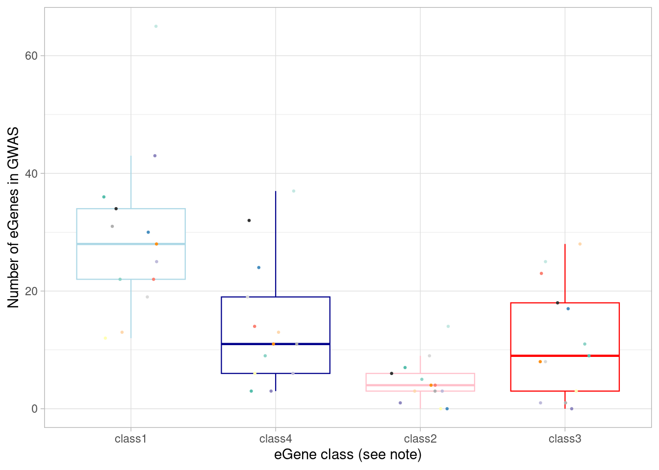
| Version | Author | Date |
|---|---|---|
| f0eaf05 | Ben Umans | 2024-09-05 |
What if we looked at fraction of the eGenes in that category instead of total numbers?
mash_by_condition_output %>%
filter(sig_anywhere) %>%
mutate(class=case_when(control10_lfsr < 0.1 & allsharing ~ "class1",
control10_lfsr < 0.1 & !allsharing ~ "class2",
sig_anywhere & control10_lfsr > 0.1 & !allsharing ~ "class3",
sig_anywhere & allsharing ~ "class4")) %>%
group_by(source, class) %>%
summarise(egene_gwas = sum(gene %in% (unlist(gwas_gene_lists) %>% unique())),
egene_in_gwas_fraction = (sum(gene %in% (unlist(gwas_gene_lists) %>% unique())))/n()) %>%
ggplot(aes(x=factor(class, levels = c("class1", "class4", "class2", "class3")), y=egene_in_gwas_fraction)) + geom_boxplot(outlier.shape = NA, aes(color=class), linewidth=0.4) +
xlab("eGene class (see note)") +
ylab("Number of eGenes in GWAS") +
theme_light() +
geom_point(aes(group=source, color=source), position = position_jitter(width = 0.2, height = 0), size=0.5) +
scale_color_manual(values=c(manual_palette_fine, class_colors)) +
xlab("eGene class (see note)") +
theme(legend.position="none")`summarise()` has grouped output by 'source'. You can override using the
`.groups` argument.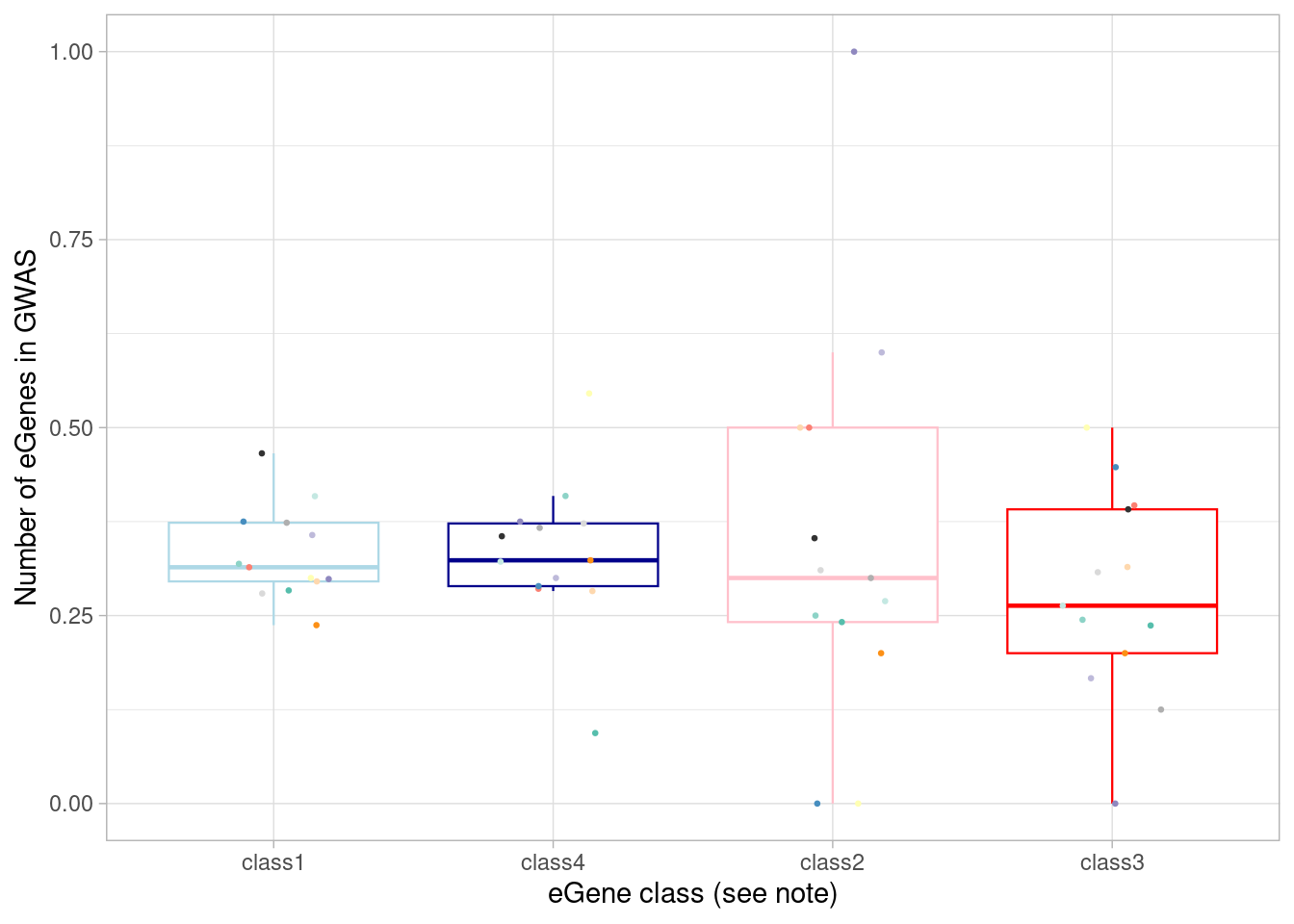 Basically the same proportion of each category.
Here, I show the numbers plotted above and perform a Wilcoxon test comparing the dynamic/not-detected-in-normoxia (“class3”) GWAS-associated eGenes with the non-dynamic/detected-in-normoxia (“class1”) GWAS-associated eGenes.
mash_by_condition_output %>%
filter(sig_anywhere) %>%
mutate(class=case_when(control10_lfsr < 0.1 & allsharing ~ "class1",
control10_lfsr < 0.1 & !allsharing ~ "class2",
sig_anywhere & control10_lfsr > 0.1 & !allsharing ~ "class3",
sig_anywhere & allsharing ~ "class4")) %>%
group_by(source, class) %>%
summarise(egene_gwas = sum(gene %in% (unlist(gwas_gene_lists) %>% unique()))) %>%
group_by(class) %>%
summarize(median(egene_gwas)) %>% kable()`summarise()` has grouped output by 'source'. You can override using the
`.groups` argument.| class | median(egene_gwas) |
|---|---|
| class1 | 28 |
| class2 | 4 |
| class3 | 9 |
| class4 | 11 |
mash_by_condition_output %>%
filter(sig_anywhere) %>%
mutate(class=case_when(control10_lfsr < 0.1 & allsharing ~ "class1",
control10_lfsr < 0.1 & !allsharing ~ "class2",
sig_anywhere & control10_lfsr > 0.1 & !allsharing ~ "class3",
sig_anywhere & allsharing ~ "class4")) %>%
group_by( class) %>%
summarise(egene_in_gwas_fraction = (sum(gene %in% (unlist(gwas_gene_lists) %>% unique())))/n())# A tibble: 4 × 2
class egene_in_gwas_fraction
<chr> <dbl>
1 class1 0.332
2 class2 0.288
3 class3 0.306
4 class4 0.318Of course, there’s a greater number of eQTLs in GWAS among the “standard” eQTLs, because there are more of them:
wilcox.test(mash_by_condition_output %>%
filter(sig_anywhere) %>%
mutate(class=case_when(control10_lfsr < 0.1 & allsharing ~ "class1",
control10_lfsr < 0.1 & !allsharing ~ "class2",
sig_anywhere & control10_lfsr > 0.1 & !allsharing ~ "class3",
sig_anywhere & allsharing ~ "class4")) %>%
complete(source, class) %>%
group_by(source, class, .drop=FALSE) %>%
summarise(egene_gwas = sum(gene %in% (unlist(gwas_gene_lists) %>% unique()))) %>%
pivot_wider(names_from = class, values_from = egene_gwas) %>% pull(class1),
mash_by_condition_output %>%
filter(sig_anywhere) %>%
mutate(class=case_when(control10_lfsr < 0.1 & allsharing ~ "class1",
control10_lfsr < 0.1 & !allsharing ~ "class2",
sig_anywhere & control10_lfsr > 0.1 & !allsharing ~ "class3",
sig_anywhere & allsharing ~ "class4")) %>%
complete(source, class) %>%
group_by(source, class, .drop=FALSE) %>%
summarise(egene_gwas = sum(gene %in% (unlist(gwas_gene_lists) %>% unique()))) %>%
pivot_wider(names_from = class, values_from = egene_gwas) %>% pull(class3), paired = TRUE)`summarise()` has grouped output by 'source'. You can override using the
`.groups` argument.
`summarise()` has grouped output by 'source'. You can override using the
`.groups` argument.Warning in wilcox.test.default(mash_by_condition_output %>%
filter(sig_anywhere) %>% : cannot compute exact p-value with ties
Wilcoxon signed rank test with continuity correction
data: mash_by_condition_output %>% filter(sig_anywhere) %>% mutate(class = case_when(control10_lfsr < 0.1 & allsharing ~ "class1", control10_lfsr < 0.1 & !allsharing ~ "class2", sig_anywhere & control10_lfsr > 0.1 & !allsharing ~ "class3", sig_anywhere & allsharing ~ "class4")) %>% complete(source, class) %>% group_by(source, class, .drop = FALSE) %>% summarise(egene_gwas = sum(gene %in% (unlist(gwas_gene_lists) %>% unique()))) %>% pivot_wider(names_from = class, values_from = egene_gwas) %>% pull(class1) and mash_by_condition_output %>% filter(sig_anywhere) %>% mutate(class = case_when(control10_lfsr < 0.1 & allsharing ~ "class1", control10_lfsr < 0.1 & !allsharing ~ "class2", sig_anywhere & control10_lfsr > 0.1 & !allsharing ~ "class3", sig_anywhere & allsharing ~ "class4")) %>% complete(source, class) %>% group_by(source, class, .drop = FALSE) %>% summarise(egene_gwas = sum(gene %in% (unlist(gwas_gene_lists) %>% unique()))) %>% pivot_wider(names_from = class, values_from = egene_gwas) %>% pull(class3)
V = 84, p-value = 0.007896
alternative hypothesis: true location shift is not equal to 0But the proportion (i.e., the yield) is the same:
wilcox.test(mash_by_condition_output %>%
filter(sig_anywhere) %>%
mutate(class=case_when(control10_lfsr < 0.1 & allsharing ~ "class1",
control10_lfsr < 0.1 & !allsharing ~ "class2",
sig_anywhere & control10_lfsr > 0.1 & !allsharing ~ "class3",
sig_anywhere & allsharing ~ "class4")) %>%
complete(source, class) %>%
group_by(source, class, .drop=FALSE) %>%
summarise(egene_in_gwas_fraction = (sum(gene %in% (unlist(gwas_gene_lists) %>% unique())))/n()) %>%
pivot_wider(names_from = class, values_from = egene_in_gwas_fraction) %>% pull(class1),
mash_by_condition_output %>%
filter(sig_anywhere) %>%
mutate(class=case_when(control10_lfsr < 0.1 & allsharing ~ "class1",
control10_lfsr < 0.1 & !allsharing ~ "class2",
sig_anywhere & control10_lfsr > 0.1 & !allsharing ~ "class3",
sig_anywhere & allsharing ~ "class4")) %>%
complete(source, class) %>%
group_by(source, class, .drop=FALSE) %>%
summarise(egene_in_gwas_fraction = (sum(gene %in% (unlist(gwas_gene_lists) %>% unique())))/n()) %>%
pivot_wider(names_from = class, values_from = egene_in_gwas_fraction) %>% pull(class3), paired = TRUE)`summarise()` has grouped output by 'source'. You can override using the
`.groups` argument.
`summarise()` has grouped output by 'source'. You can override using the
`.groups` argument.
Wilcoxon signed rank exact test
data: mash_by_condition_output %>% filter(sig_anywhere) %>% mutate(class = case_when(control10_lfsr < 0.1 & allsharing ~ "class1", control10_lfsr < 0.1 & !allsharing ~ "class2", sig_anywhere & control10_lfsr > 0.1 & !allsharing ~ "class3", sig_anywhere & allsharing ~ "class4")) %>% complete(source, class) %>% group_by(source, class, .drop = FALSE) %>% summarise(egene_in_gwas_fraction = (sum(gene %in% (unlist(gwas_gene_lists) %>% unique())))/n()) %>% pivot_wider(names_from = class, values_from = egene_in_gwas_fraction) %>% pull(class1) and mash_by_condition_output %>% filter(sig_anywhere) %>% mutate(class = case_when(control10_lfsr < 0.1 & allsharing ~ "class1", control10_lfsr < 0.1 & !allsharing ~ "class2", sig_anywhere & control10_lfsr > 0.1 & !allsharing ~ "class3", sig_anywhere & allsharing ~ "class4")) %>% complete(source, class) %>% group_by(source, class, .drop = FALSE) %>% summarise(egene_in_gwas_fraction = (sum(gene %in% (unlist(gwas_gene_lists) %>% unique())))/n()) %>% pivot_wider(names_from = class, values_from = egene_in_gwas_fraction) %>% pull(class3)
V = 64, p-value = 0.2163
alternative hypothesis: true location shift is not equal to 0Overall (ie, not per-cell type):
mash_by_condition_output %>%
filter(sig_anywhere) %>%
mutate(class=case_when(control10_lfsr < 0.1 & allsharing ~ "class1",
control10_lfsr < 0.1 & !allsharing ~ "class2",
sig_anywhere & control10_lfsr > 0.1 & !allsharing ~ "class3",
sig_anywhere & allsharing ~ "class4")) %>%
select(gene, class) %>%
distinct() %>%
group_by(class) %>%
summarise(egene_gwas = sum(gene %in% (unlist(gwas_gene_lists) %>% unique()))) %>%
kable()| class | egene_gwas |
|---|---|
| class1 | 291 |
| class2 | 59 |
| class3 | 148 |
| class4 | 175 |
The same numbers can be calculated excluding genes that have already been identified as eGenes in GTEx cerebral cortex tissue.
mash_by_condition_output %>%
filter(sig_anywhere) %>%
filter(gene %not_in% gtex_cortex_signif) %>%
mutate(class=case_when(control10_lfsr < 0.1 & allsharing ~ "class1",
control10_lfsr < 0.1 & !allsharing ~ "class2",
sig_anywhere & control10_lfsr > 0.1 & !allsharing ~ "class3",
sig_anywhere & allsharing ~ "class4")) %>%
group_by(source, class) %>%
summarise(egene_gwas = sum(gene %in% (unlist(gwas_gene_lists) %>% unique()))) %>%
group_by(class) %>%
summarize(median(egene_gwas))`summarise()` has grouped output by 'source'. You can override using the
`.groups` argument.# A tibble: 4 × 2
class `median(egene_gwas)`
<chr> <int>
1 class1 15
2 class2 2
3 class3 5
4 class4 8Overall (ie, not per-cell type):
mash_by_condition_output %>%
filter(sig_anywhere) %>%
filter(gene %not_in% gtex_cortex_signif) %>%
mutate(class=case_when(control10_lfsr < 0.1 & allsharing ~ "class1",
control10_lfsr < 0.1 & !allsharing ~ "class2",
sig_anywhere & control10_lfsr > 0.1 & !allsharing ~ "class3",
sig_anywhere & allsharing ~ "class4")) %>%
select(gene, class) %>%
distinct() %>%
group_by(class) %>%
summarise(egene_gwas = sum(gene %in% (unlist(gwas_gene_lists) %>% unique()))) %>%
kable()| class | egene_gwas |
|---|---|
| class1 | 171 |
| class2 | 32 |
| class3 | 96 |
| class4 | 108 |
To test whether the “dynamic” vs “standard” eGenes (defined solely by comparisons of effect size) are more likely to be present in GWAS gene lists, we group and test them as we did for comparison to GTEx. Note this yields a similar conclusion as above, where we broke eGenes down by whether they were dynamic and detectable at baseline.
wilcox.test(mash_by_condition_output %>%
filter(sig_anywhere) %>%
mutate(class=case_when(allsharing ~ "standard",
hypoxia_normoxia_shared & sharing_contexts==1 ~ "dynamic",
hyperoxia_normoxia_shared & sharing_contexts==1 ~ "dynamic",
hypoxia_hyperoxia_shared & sharing_contexts==1 ~ "dynamic",
sharing_contexts==2 ~ "standard",
sharing_contexts==0 ~ "dynamic"
)) %>%
complete(source, class) %>%
group_by(source, class, .drop=FALSE) %>%
summarise(egene_gwas = sum(gene %in% (unlist(gwas_gene_lists) %>% unique()))) %>%
filter(class %in% c("dynamic")) %>% pull(egene_gwas),
mash_by_condition_output %>%
filter(sig_anywhere) %>%
mutate(class=case_when(allsharing ~ "standard",
hypoxia_normoxia_shared & sharing_contexts==1 ~ "dynamic",
hyperoxia_normoxia_shared & sharing_contexts==1 ~ "dynamic",
hypoxia_hyperoxia_shared & sharing_contexts==1 ~ "dynamic",
sharing_contexts==2 ~ "standard",
sharing_contexts==0 ~ "dynamic"
)) %>%
complete(source, class) %>%
group_by(source, class, .drop=FALSE) %>%
summarise(egene_gwas = sum(gene %in% (unlist(gwas_gene_lists) %>% unique()))) %>%
filter(class %in% c("standard")) %>% pull(egene_gwas), paired=TRUE, alternative = "two.sided")`summarise()` has grouped output by 'source'. You can override using the
`.groups` argument.
`summarise()` has grouped output by 'source'. You can override using the
`.groups` argument.
Wilcoxon signed rank exact test
data: mash_by_condition_output %>% filter(sig_anywhere) %>% mutate(class = case_when(allsharing ~ "standard", hypoxia_normoxia_shared & sharing_contexts == 1 ~ "dynamic", hyperoxia_normoxia_shared & sharing_contexts == 1 ~ "dynamic", hypoxia_hyperoxia_shared & sharing_contexts == 1 ~ "dynamic", sharing_contexts == 2 ~ "standard", sharing_contexts == 0 ~ "dynamic")) %>% complete(source, class) %>% group_by(source, class, .drop = FALSE) %>% summarise(egene_gwas = sum(gene %in% (unlist(gwas_gene_lists) %>% unique()))) %>% filter(class %in% c("dynamic")) %>% pull(egene_gwas) and mash_by_condition_output %>% filter(sig_anywhere) %>% mutate(class = case_when(allsharing ~ "standard", hypoxia_normoxia_shared & sharing_contexts == 1 ~ "dynamic", hyperoxia_normoxia_shared & sharing_contexts == 1 ~ "dynamic", hypoxia_hyperoxia_shared & sharing_contexts == 1 ~ "dynamic", sharing_contexts == 2 ~ "standard", sharing_contexts == 0 ~ "dynamic")) %>% complete(source, class) %>% group_by(source, class, .drop = FALSE) %>% summarise(egene_gwas = sum(gene %in% (unlist(gwas_gene_lists) %>% unique()))) %>% filter(class %in% c("standard")) %>% pull(egene_gwas)
V = 0, p-value = 0.0002441
alternative hypothesis: true location shift is not equal to 0Compare to coarse-clustered results
mash_by_condition_output_coarse <- readRDS(file = "/project2/gilad/umans/oxygen_eqtl/output/combined_mash-by-condition_EE_coarse_reharmonized_newmash_032024.rds") %>% ungroup()Again, I plot the number of eGenes of each these four classes that are the nearest genes to a significant GWAS variant in each cell type.
mash_by_condition_output_coarse %>%
filter(sig_anywhere) %>%
mutate(class=case_when(control10_lfsr < 0.1 & allsharing ~ "class1",
control10_lfsr < 0.1 & !allsharing ~ "class2",
sig_anywhere & control10_lfsr > 0.1 & !allsharing ~ "class3",
sig_anywhere & allsharing ~ "class4")) %>%
group_by(source, class) %>%
summarise(egene_gwas = sum(gene %in% (unlist(gwas_gene_lists) %>% unique()))) %>%
ggplot(aes(x=factor(class, levels = c("class1", "class4", "class2", "class3")), y=egene_gwas)) + geom_boxplot(outlier.shape = NA, aes(color=class), linewidth=0.4) +
xlab("eGene class (see note)") +
ylab("Number of eGenes in GWAS") +
theme_light() +
geom_point(aes(group=source, color=source), position = position_jitter(width = 0.2, height = 0), size=0.5) +
scale_color_manual(values=c(manual_palette_coarse, class_colors)) +
xlab("eGene class (see note)") +
theme(legend.position="none")`summarise()` has grouped output by 'source'. You can override using the
`.groups` argument.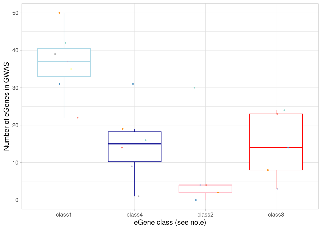
Here, I show the numbers plotted above and perform a Wilcoxon test comparing the dynamic/not-detected-in-normoxia (“class3”) GWAS-associated eGenes with the non-dynamic/detected-in-normoxia (“class1”) GWAS-associated eGenes.
mash_by_condition_output_coarse %>%
filter(sig_anywhere) %>%
mutate(class=case_when(control10_lfsr < 0.1 & allsharing ~ "class1",
control10_lfsr < 0.1 & !allsharing ~ "class2",
sig_anywhere & control10_lfsr > 0.1 & !allsharing ~ "class3",
sig_anywhere & allsharing ~ "class4")) %>%
group_by(source, class) %>%
summarise(egene_gwas = sum(gene %in% (unlist(gwas_gene_lists) %>% unique()))) %>%
group_by(class) %>%
summarize(median(egene_gwas)) %>% kable()`summarise()` has grouped output by 'source'. You can override using the
`.groups` argument.| class | median(egene_gwas) |
|---|---|
| class1 | 37 |
| class2 | 4 |
| class3 | 14 |
| class4 | 15 |
wilcox.test(mash_by_condition_output_coarse %>%
filter(sig_anywhere) %>%
mutate(class=case_when(control10_lfsr < 0.1 & allsharing ~ "class1",
control10_lfsr < 0.1 & !allsharing ~ "class2",
sig_anywhere & control10_lfsr > 0.1 & !allsharing ~ "class3",
sig_anywhere & allsharing ~ "class4")) %>%
complete(source, class) %>%
group_by(source, class, .drop=FALSE) %>%
summarise(egene_gwas = sum(gene %in% (unlist(gwas_gene_lists) %>% unique()))) %>%
pivot_wider(names_from = class, values_from = egene_gwas) %>% pull(class1),
mash_by_condition_output_coarse %>%
filter(sig_anywhere) %>%
mutate(class=case_when(control10_lfsr < 0.1 & allsharing ~ "class1",
control10_lfsr < 0.1 & !allsharing ~ "class2",
sig_anywhere & control10_lfsr > 0.1 & !allsharing ~ "class3",
sig_anywhere & allsharing ~ "class4")) %>%
complete(source, class) %>%
group_by(source, class, .drop=FALSE) %>%
summarise(egene_gwas = sum(gene %in% (unlist(gwas_gene_lists) %>% unique()))) %>%
pivot_wider(names_from = class, values_from = egene_gwas) %>% pull(class3), paired = TRUE)`summarise()` has grouped output by 'source'. You can override using the
`.groups` argument.
`summarise()` has grouped output by 'source'. You can override using the
`.groups` argument.Warning in wilcox.test.default(mash_by_condition_output_coarse %>%
filter(sig_anywhere) %>% : cannot compute exact p-value with ties
Wilcoxon signed rank test with continuity correction
data: mash_by_condition_output_coarse %>% filter(sig_anywhere) %>% mutate(class = case_when(control10_lfsr < 0.1 & allsharing ~ "class1", control10_lfsr < 0.1 & !allsharing ~ "class2", sig_anywhere & control10_lfsr > 0.1 & !allsharing ~ "class3", sig_anywhere & allsharing ~ "class4")) %>% complete(source, class) %>% group_by(source, class, .drop = FALSE) %>% summarise(egene_gwas = sum(gene %in% (unlist(gwas_gene_lists) %>% unique()))) %>% pivot_wider(names_from = class, values_from = egene_gwas) %>% pull(class1) and mash_by_condition_output_coarse %>% filter(sig_anywhere) %>% mutate(class = case_when(control10_lfsr < 0.1 & allsharing ~ "class1", control10_lfsr < 0.1 & !allsharing ~ "class2", sig_anywhere & control10_lfsr > 0.1 & !allsharing ~ "class3", sig_anywhere & allsharing ~ "class4")) %>% complete(source, class) %>% group_by(source, class, .drop = FALSE) %>% summarise(egene_gwas = sum(gene %in% (unlist(gwas_gene_lists) %>% unique()))) %>% pivot_wider(names_from = class, values_from = egene_gwas) %>% pull(class3)
V = 27, p-value = 0.03429
alternative hypothesis: true location shift is not equal to 0Note that, in the coarsely-clustered data, more GWAS-associated eGenes appear non-dynamic (ie, have equivalent responses across oxygen conditions) and fewer appear context-specific.
The same numbers can be calculated excluding genes that have already been identified as eGenes in GTEx cerebral cortex tissue.
mash_by_condition_output_coarse %>%
filter(sig_anywhere) %>%
filter(gene %not_in% gtex_cortex_signif) %>%
mutate(class=case_when(control10_lfsr < 0.1 & allsharing ~ "class1",
control10_lfsr < 0.1 & !allsharing ~ "class2",
sig_anywhere & control10_lfsr > 0.1 & !allsharing ~ "class3",
sig_anywhere & allsharing ~ "class4")) %>%
group_by(source, class) %>%
summarise(egene_gwas = sum(gene %in% (unlist(gwas_gene_lists) %>% unique()))) %>%
group_by(class) %>%
summarize(median(egene_gwas))`summarise()` has grouped output by 'source'. You can override using the
`.groups` argument.# A tibble: 4 × 2
class `median(egene_gwas)`
<chr> <dbl>
1 class1 20
2 class2 2
3 class3 9
4 class4 10What if we looked at fraction of the eGenes in that category instead of total numbers?
mash_by_condition_output_coarse %>%
filter(sig_anywhere) %>%
mutate(class=case_when(control10_lfsr < 0.1 & allsharing ~ "class1",
control10_lfsr < 0.1 & !allsharing ~ "class2",
sig_anywhere & control10_lfsr > 0.1 & !allsharing ~ "class3",
sig_anywhere & allsharing ~ "class4")) %>%
group_by(source, class) %>%
summarise(egene_gwas = sum(gene %in% (unlist(gwas_gene_lists) %>% unique())),
egene_in_gwas_fraction = (sum(gene %in% (unlist(gwas_gene_lists) %>% unique())))/n()) %>%
ggplot(aes(x=factor(class, levels = c("class1", "class4", "class2", "class3")), y=egene_in_gwas_fraction)) + geom_boxplot(outlier.shape = NA, aes(color=class), linewidth=0.4) +
xlab("eGene class (see note)") +
ylab("Number of eGenes in GWAS") +
theme_light() +
geom_point(aes(group=source, color=source), position = position_jitter(width = 0.2, height = 0), size=0.5) +
scale_color_manual(values=c(manual_palette_fine, class_colors)) +
xlab("eGene class (see note)") +
theme(legend.position="none")`summarise()` has grouped output by 'source'. You can override using the
`.groups` argument.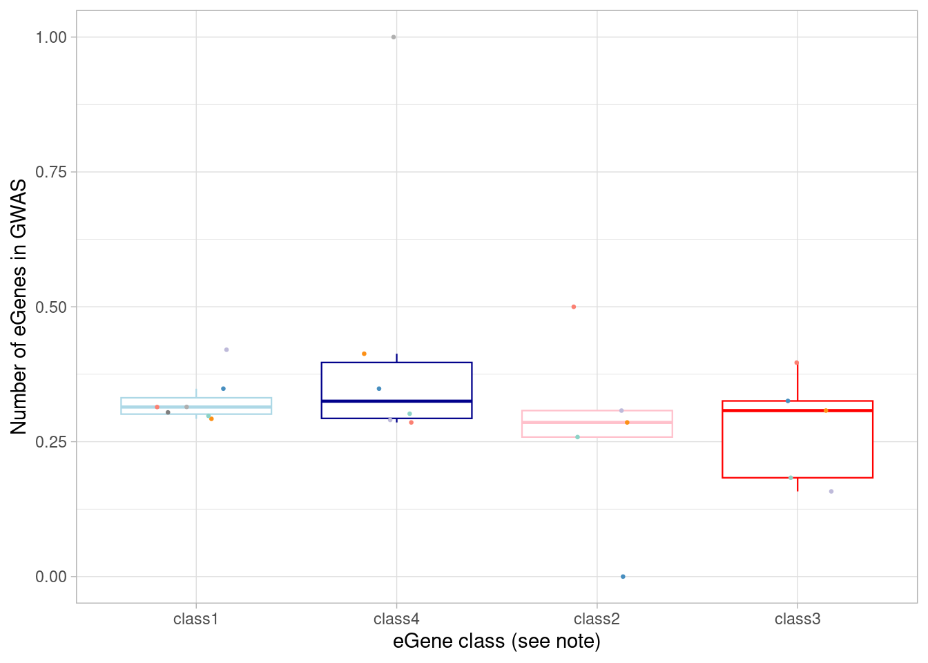 Basically the same proportion of each category.
To test whether the “dynamic” vs “standard” eGenes (defined solely by comparisons of effect size) are more likely to be present in GWAS gene lists, we group and test them as we did for comparison to GTEx. Note this yields a similar conclusion as above, where we broke eGenes down by whether they were dynamic and detectable at baseline.
wilcox.test(mash_by_condition_output_coarse %>%
filter(sig_anywhere) %>%
mutate(class=case_when(allsharing ~ "standard",
hypoxia_normoxia_shared & sharing_contexts==1 ~ "dynamic",
hyperoxia_normoxia_shared & sharing_contexts==1 ~ "dynamic",
hypoxia_hyperoxia_shared & sharing_contexts==1 ~ "dynamic",
sharing_contexts==2 ~ "standard",
sharing_contexts==0 ~ "dynamic"
)) %>%
complete(source, class) %>%
group_by(source, class, .drop=FALSE) %>%
summarise(egene_gwas = sum(gene %in% (unlist(gwas_gene_lists) %>% unique()))) %>% filter(class %in% c("dynamic")) %>% pull(egene_gwas),
mash_by_condition_output_coarse %>%
filter(sig_anywhere) %>%
mutate(class=case_when(allsharing ~ "standard",
hypoxia_normoxia_shared & sharing_contexts==1 ~ "dynamic",
hyperoxia_normoxia_shared & sharing_contexts==1 ~ "dynamic",
hypoxia_hyperoxia_shared & sharing_contexts==1 ~ "dynamic",
sharing_contexts==2 ~ "standard",
sharing_contexts==0 ~ "dynamic"
)) %>%
complete(source, class) %>%
group_by(source, class, .drop=FALSE) %>%
summarise(egene_gwas = sum(gene %in% (unlist(gwas_gene_lists) %>% unique()))) %>% filter(class %in% c("standard")) %>% pull(egene_gwas), paired=TRUE, alternative = "two.sided")`summarise()` has grouped output by 'source'. You can override using the
`.groups` argument.
`summarise()` has grouped output by 'source'. You can override using the
`.groups` argument.
    Wilcoxon signed rank exact test

data:  mash_by_condition_output_coarse %>% filter(sig_anywhere) %>% mutate(class = case_when(allsharing ~ "standard", hypoxia_normoxia_shared & sharing_contexts == 1 ~ "dynamic", hyperoxia_normoxia_shared & sharing_contexts == 1 ~ "dynamic", hypoxia_hyperoxia_shared & sharing_contexts == 1 ~ "dynamic", sharing_contexts == 2 ~ "standard", sharing_contexts == 0 ~ "dynamic")) %>% complete(source, class) %>% group_by(source, class, .drop = FALSE) %>% summarise(egene_gwas = sum(gene %in% (unlist(gwas_gene_lists) %>%      unique()))) %>% filter(class %in% c("dynamic")) %>% pull(egene_gwas) and mash_by_condition_output_coarse %>% filter(sig_anywhere) %>% mutate(class = case_when(allsharing ~ "standard", hypoxia_normoxia_shared & sharing_contexts == 1 ~ "dynamic", hyperoxia_normoxia_shared & sharing_contexts == 1 ~ "dynamic", hypoxia_hyperoxia_shared & sharing_contexts == 1 ~ "dynamic", sharing_contexts == 2 ~ "standard", sharing_contexts == 0 ~ "dynamic")) %>% complete(source, class) %>% group_by(source, class, .drop = FALSE) %>% summarise(egene_gwas = sum(gene %in% (unlist(gwas_gene_lists) %>%      unique()))) %>% filter(class %in% c("standard")) %>% pull(egene_gwas)
V = 0, p-value = 0.01563
alternative hypothesis: true location shift is not equal to 0
Topic-interacting eQTL results
Finally, compare the topic-interacting eQTL genes to the GWAS gene list. Obtain the topic 7-correlated eGenes the same as shown previously:
crm_signif <- vroom("/project2/gilad/umans/oxygen_eqtl/topicqtl/outputs/topics15/all_genes_merged_fine_fasttopics_15_topics.cellregmap.sighits.tsv")Rows: 289 Columns: 5
── Column specification ────────────────────────────────────────────────────────
Delimiter: "\t"
chr (2): GENE_HGNC, VARIANT_ID
dbl (3): P_CELLREGMAP, P_BONF, q
ℹ Use `spec()` to retrieve the full column specification for this data.
ℹ Specify the column types or set `show_col_types = FALSE` to quiet this message.crm_iegenes <- crm_signif$GENE_HGNC
crm_betas <- vroom(paste0("/project2/gilad/umans/oxygen_eqtl/topicqtl/outputs/topics15/fasttopics_fine_15_topics.", crm_iegenes, ".cellregmap.betas.tsv"))Rows: 3094323 Columns: 5
── Column specification ────────────────────────────────────────────────────────
Delimiter: "\t"
chr (3): PSEUDOCELL, GENE_HGNC, VARIANT_ID
dbl (2): BETA_GXC, BETA_G
ℹ Use `spec()` to retrieve the full column specification for this data.
ℹ Specify the column types or set `show_col_types = FALSE` to quiet this message.crm_betas_wide <- dplyr::select(crm_betas, c(PSEUDOCELL, BETA_GXC, GENE_HGNC, VARIANT_ID)) %>%
unite(TOPIC_QTL, GENE_HGNC, VARIANT_ID, sep="_") %>%
pivot_wider(id_cols=PSEUDOCELL, names_from=TOPIC_QTL, values_from=BETA_GXC)
topic_loadings <- vroom("/project2/gilad/umans/oxygen_eqtl/topicqtl/pseudocell_loadings_k15.tsv")Rows: 10707 Columns: 16
── Column specification ────────────────────────────────────────────────────────
Delimiter: "\t"
chr (1): pseudocell
dbl (15): k1, k2, k3, k4, k5, k6, k7, k8, k9, k10, k11, k12, k13, k14, k15
ℹ Use `spec()` to retrieve the full column specification for this data.
ℹ Specify the column types or set `show_col_types = FALSE` to quiet this message.crm_betas_loadings <- left_join(crm_betas_wide, topic_loadings, by=c("PSEUDOCELL"="pseudocell"))
beta_topic_corrs_matrix <- cor(dplyr::select(crm_betas_loadings, -c(PSEUDOCELL, paste0("k", seq(15)))),
dplyr::select(crm_betas_loadings, paste0("k", seq(15))))
beta_topic_corrs_p <- apply(dplyr::select(crm_betas_loadings, -c(PSEUDOCELL, paste0("k", seq(15)))) %>% as.matrix(), MARGIN = 2, FUN = function(x) cor.test(x, crm_betas_loadings$k7)$p.value )
k7_egenes <- beta_topic_corrs_matrix %>% as.data.frame() %>%
dplyr::select(k7) %>%
bind_cols(beta_topic_corrs_p) %>%
rownames_to_column(var = "gene_snp") %>%
separate(gene_snp, into = c("genename", "snp"), sep = "_") %>%
mutate(snp_short = str_sub(snp, end = -5)) %>%
filter(`...2` < (0.05/289)) %>% pull(genename)New names:
• `` -> `...2`Now, intersect with GWAS genes:
sum(k7_egenes %in% (unlist(gwas_gene_lists) %>% unique()))[1] 55If we exclude the genes in GTEx cortex samples:
length(intersect(setdiff(k7_egenes, gtex_cortex_signif), (unlist(gwas_gene_lists) %>% unique())))[1] 31How many are not included in our pseudobulk-identified set of hypoxia-specific eGenes?
hypoxia_egenes <- mash_by_condition_output %>%
  filter(sig_anywhere) %>%
 mutate(class=case_when(allsharing ~ "allsharing",
                        hypoxia_normoxia_shared & sharing_contexts==1 ~ "hyperoxia_specific",
                        hyperoxia_normoxia_shared & sharing_contexts==1 ~ "hypoxia_specific",
                        hypoxia_hyperoxia_shared & sharing_contexts==1 ~ "normoxia_specific",
                        sharing_contexts==2 ~ "partial_shared",
                        sharing_contexts==0 ~ "alldiff"
                        )) %>%
  filter(class=="hypoxia_specific") %>%
  pull(gene) %>%
  unique()

any_egenes <- mash_by_condition_output %>%
  filter(sig_anywhere) %>%
  pull(gene) %>%
  unique()

length(setdiff(k7_egenes, hypoxia_egenes))
[1] 214length(setdiff(k7_egenes, any_egenes))[1] 150Process rare variant results
Here, I import datasets downloaded from SCHEMA, BipEx, Epi25, DDD, and SFARI Genes.
schema <- read.table(file = "/project2/gilad/umans/oxygen_eqtl/data/external/SCHEMA_gene_results.txt", header = TRUE, sep = "\t", stringsAsFactors = FALSE)
# convert to gene symbols
bipex <- read.table(file = "/project2/gilad/umans/oxygen_eqtl/data/external/BipEx_gene_results_new.tsv", header = TRUE, sep = "\t", stringsAsFactors = FALSE)
# convert to gene symbols
epi25 <- read.table(file = "/project2/gilad/umans/oxygen_eqtl/data/external/Epi25_gene_results.tsv", header = TRUE, sep = "\t", stringsAsFactors = FALSE)
# convert to gene symbols
ddd <- read.csv(file = "/project2/gilad/umans/oxygen_eqtl/data/external/DDD_gene_results.csv", header = TRUE, stringsAsFactors = FALSE)
sfari <- read.csv(file = "/project2/gilad/umans/oxygen_eqtl/data/external/SFARI-Gene_genes.csv", header = TRUE,  stringsAsFactors = FALSE)
Change the ensembl gene names in the SCHEMA, BipEx, and Epi25 sets:
library(GenomicRanges)
gene.gr <- readRDS('/project/gilad/umans/brainchromatin/data_files/rds/AllGenes_GenomicRanges.RDS')

convertGeneIDs <- function(genelist, id.mapping.table) {
  return(mapValues(x = genelist, mapping.table = id.mapping.table))
}
mapValues <- function(x,mapping.table) {
  out <- mapping.table[x]
  if(any(is.na(out))) {
    na <- sum(is.na(out))
    cat(sprintf("Warning: mapping returned %s NA values\n", as.character(na)))
  }
  return(out)
}

name2ensembl <- names(gene.gr)

# Something funny about this one, unsure why yet
name2ensembl['CDR1'] <- 'ENSG00000281508'

names(name2ensembl) <- elementMetadata(gene.gr)[ ,'gene_name']

ensembl2name <- elementMetadata(gene.gr)[ ,'gene_name']
names(ensembl2name) <- names(gene.gr)

schema$gene_name <- unname(convertGeneIDs(schema$gene_id, ensembl2name))
Warning: mapping returned 222 NA valuesbipex$gene_name <- unname(convertGeneIDs(bipex$gene_id, ensembl2name))Warning: mapping returned 684 NA valuesepi25$gene_name <- unname(convertGeneIDs(epi25$gene_id, ensembl2name))Warning: mapping returned 28 NA valuesCompile results into a list.
rare_gene_list <- list(bipex= bipex %>%
                         filter(group=="Bipolar Disorder") %>%
                         filter(damaging_missense_fisher_gnom_non_psych_pval<0.05|ptv_fisher_gnom_non_psych_pval<0.05) %>%
                         drop_na(gene_name) %>%
                         pull(gene_name),
                       epi25 = epi25 %>% filter(group=="EPI") %>%
                         filter(ptv_pval<0.05) %>%
                         drop_na(gene_name) %>%
                         pull(gene_name),
                       schema = schema %>% filter(Qmeta<0.05) %>%
                         drop_na(gene_name) %>%
                         pull(gene_name),
                       sfari_asd = sfari %>% filter(gene.score==1) %>%
                         pull(gene.symbol),
                       sfari_syndromic = sfari %>% filter(syndromic==1) %>%
                         pull(gene.symbol),
                       ddd= ddd %>% filter(significant) %>% pull(symbol)
                       )
Pleiotropy in psychiatric genetics is well documented. Are the genes pulled from each of these sources largely unique?
length(unique(unlist(rare_gene_list)))/length(unlist(rare_gene_list))[1] 0.8132296Yes, about 81% of the genes here are not redundant across studies.
Compile the same results into a data frame.
rare_gene_frame <- rbind(data.frame(source= "bipex", gene= bipex %>%
                         filter(group=="Bipolar Disorder") %>%
                         filter(damaging_missense_fisher_gnom_non_psych_pval<0.05|ptv_fisher_gnom_non_psych_pval<0.05) %>%
                         drop_na(gene_name) %>%
                         pull(gene_name)),
                         data.frame(source="epi25", gene = epi25 %>% filter(group=="EPI") %>%
                         filter(ptv_pval<0.05) %>%
                         drop_na(gene_name) %>%
                         pull(gene_name)),
                         data.frame(source= "schema", gene = schema %>% filter(Qmeta<0.05) %>%
                         drop_na(gene_name) %>%
                         pull(gene_name)),
                         data.frame(source= "sfari_asd", gene = sfari %>% filter(gene.score==1) %>%
                         pull(gene.symbol)),
                       data.frame(source="sfari_syndromic", gene = sfari %>% filter(syndromic==1) %>%
                         pull(gene.symbol)),
                       data.frame(source= "ddd", gene= ddd %>% filter(significant) %>% pull(symbol)))
Now, just like above for GWAS genes, compare each eGene class to rare variant genes in each cell type.
mash_by_condition_output %>%
  filter(sig_anywhere) %>%
  mutate(class=case_when(control10_lfsr < 0.1 & allsharing ~ "class1",
                         control10_lfsr < 0.1 &  !allsharing ~ "class2",
                         sig_anywhere & control10_lfsr > 0.1 & !allsharing ~ "class3",
                         sig_anywhere & allsharing ~ "class4")) %>%
   group_by(source, class) %>%
  summarise(egene_rare = sum(gene %in% (unlist(rare_gene_frame$gene) %>% unique()))) %>%
  ggplot(aes(x=factor(class, levels = c("class1", "class4", "class2", "class3")), y=egene_rare)) +
  geom_boxplot(outlier.shape = NA, aes(color=class)) +
  ylab("Rare variant genes with eQTLs") +
  theme_light() +
  geom_point(aes(group=source, color=source), position = position_jitter(width = 0.2, height = 0)) +
  scale_color_manual(values=c(manual_palette_fine, class_colors)) +
  xlab("eGene class (see note)") +
  theme(legend.position="none")
`summarise()` has grouped output by 'source'. You can override using the
`.groups` argument.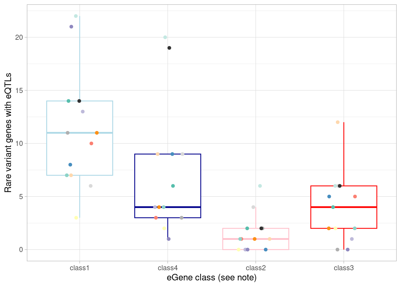
| Version | Author | Date |
|---|---|---|
| f0eaf05 | Ben Umans | 2024-09-05 |
# additionally, compare to GWAS results as above, but first restricting to rare variant-associated genes.
mash_by_condition_output %>%
  filter(sig_anywhere) %>%
  filter(gene %in% rare_gene_frame$gene) %>%
  mutate(class=case_when(control10_lfsr < 0.1 & allsharing ~ "class1",
                         control10_lfsr < 0.1 &  !allsharing ~ "class2",
                         sig_anywhere & control10_lfsr > 0.1 & !allsharing ~ "class3",
                         sig_anywhere & allsharing ~ "class4")) %>%
  group_by(source, class) %>%
  summarise(egene_rare = sum(gene %in% (unlist(gwas_gene_lists) %>% unique()))) %>%
  ggplot(aes(x=factor(class, levels = c("class1", "class4", "class2", "class3")), y=egene_rare)) +
  geom_boxplot(outlier.shape = NA, aes(color=class), linewidth=0.4) +
  xlab("eGene class (see note") +
  ylab("Rare variant genes with GWAS eQTLs") +
  theme_light() +
  scale_color_manual(values=c(manual_palette_fine, class_colors)) +
  theme(legend.position="none") +
  geom_point(aes(group=source, color=source), position = position_jitter(width = 0.2, height = 0), size=0.5)
`summarise()` has grouped output by 'source'. You can override using the
`.groups` argument.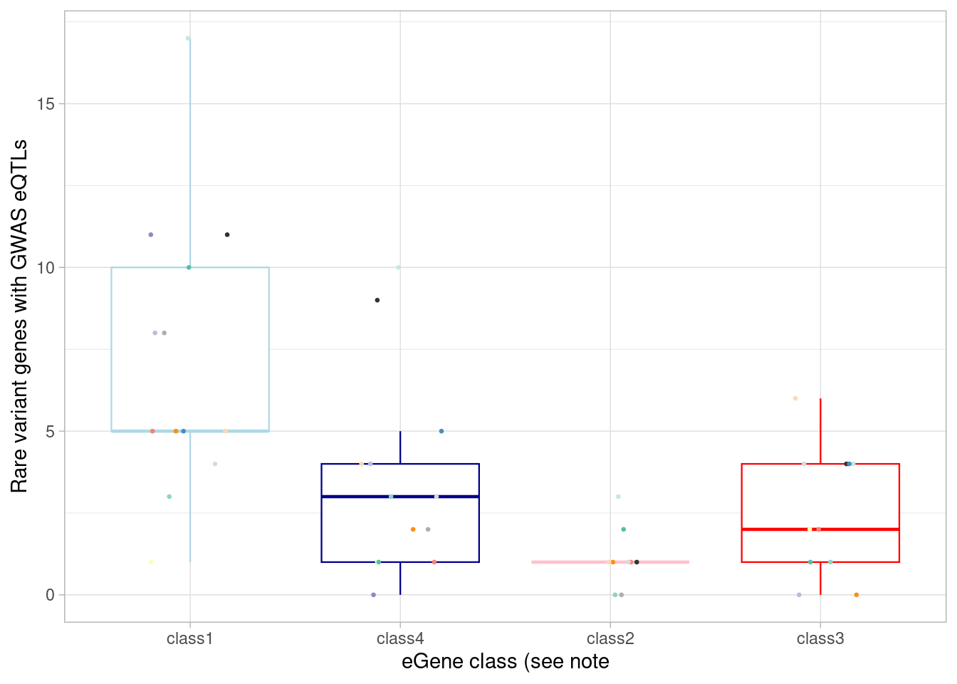
The total number of rare variant genes with an eQTL is:
mash_by_condition_output %>%
  filter(sig_anywhere) %>%
  filter(gene %in% rare_gene_frame$gene) %>%
  pull(gene) %>%
  unique() %>%
  length()
[1] 225The total number of rare variant genes with an eQTL that correspond to one of our GWAS traits is:
mash_by_condition_output %>%
  filter(sig_anywhere) %>%
  filter(gene %in% rare_gene_frame$gene) %>%
  filter(gene %in% (unlist(gwas_gene_lists) %>% unique())) %>%
  pull(gene) %>%
  unique() %>%
  length()
[1] 123Rare variant genes that are eGenes in our dataset allow us to ask about the phenotypic consequences of modulating expression levels of genes for which loss of function has an identified phenotype, linked together by a SNP. Here, we can join those together, bridging the GWAS results and the rare variant results by our eQTL results. Note that this is of course an underestimate of this analysis, since we’re only using those SNPs chosen as lead variants by mash which are themselves GWAS hits. There may be other equivalent or secondary SNPs masked by mash here that still provide information.
inner_join(x=mash_by_condition_output %>%
# filter(sig_anywhere) %>%
  filter(control10_lfsr < 0.2 | stim1pct_lfsr < 0.2 | stim21pct_lfsr < 0.2 ) %>%
  filter(gene %in% rare_gene_frame$gene) %>%
  mutate(class=case_when(control10_lfsr < 0.2 & allsharing ~ "class1",
                         control10_lfsr < 0.2 &  !allsharing ~ "class2",
                         control10_lfsr > 0.2 & !allsharing ~ "class3",
                         allsharing ~ "class4")) %>%
  separate(gene_snp, into = c("genename", "snp"), sep = "_") %>%
    mutate(snp_short = str_sub(snp, end = -5)) %>%
    select(gene, snp, snp_short, source, control10_lfsr:stim21pct_beta, class),
  y=gwas_formatted %>% filter(trait %in% filtered_traits) %>% filter(n>15) %>% filter(n<500) %>%
  filter(PVALUE_MLOG>7.3) %>% unite("snp", CHR_ID:CHR_POS, sep = ":") %>% select(nearest_gene, REPORTED.GENE.S., trait, n, snp, STUDY.ACCESSION, PVALUE_MLOG, UPSTREAM_GENE_DISTANCE, DOWNSTREAM_GENE_DISTANCE) ,
  by=join_by(snp_short==snp), relationship = "many-to-many")  %>%
  mutate(across(ends_with("lfsr"), signif)) %>%
  mutate(across(ends_with("beta"), signif)) %>%
  select(gene, source, class, snp, nearest_gene, STUDY.ACCESSION, trait) %>%
  left_join(x=., y=rare_gene_frame, by=join_by(gene==gene), relationship = "many-to-many")
gene source.x class snp nearest_gene STUDY.ACCESSION
1 NRXN3 Glut class1 14:78164146:C:G NRXN3 GCST90267280
2 CUL3 InhGNRH class3 2:224608546:C:T CUL3 GCST90239693
3 CTTNBP2 InhThalamic class4 7:117883655:A:G CTTNBP2 GCST005324
4 CTTNBP2 InhThalamic class4 7:117883655:A:G CTTNBP2 GCST008810
5 CTTNBP2 InhThalamic class4 7:117883655:A:G CTTNBP2 GCST007474
6 CTTNBP2 InhThalamic class4 7:117883655:A:G CTTNBP2 GCST007462
7 CTTNBP2 InhThalamic class4 7:117883655:A:G CTTNBP2 GCST007085
8 SCN1A NeuronOther class1 2:166142257:C:G SCN3A GCST007343
9 SCN1A NeuronOther class1 2:166142257:C:G SCN3A GCST007343
10 SCN1A NeuronOther class1 2:166142257:C:G SCN3A GCST007343
11 SCN1A NeuronOther class1 2:166142257:C:G SCN3A GCST007343
12 GNAO1 RG class1 16:56227517:T:G GNAO1 GCST007982
13 POU3F3 RGcycling class1 2:104849547:G:A PANTR1 GCST90012894
14 POU3F3 RGcycling class1 2:104849547:G:A PANTR1 GCST90012894
15 POU3F3 RGcycling class1 2:104849547:G:A PANTR1 GCST90131905
16 POU3F3 RGcycling class1 2:104849547:G:A PANTR1 GCST90131905
trait
1 Age when finished full-time education (standard GWA)
2 Risk-taking behavior (multivariate analysis)
3 Depressive symptoms
4 Smoking initiation (ever regular vs never regular)
5 Smoking initiation (ever regular vs never regular)
6 Age of smoking initiation (MTAG)
7 Smoking status
8 Epilepsy
9 Epilepsy
10 Epilepsy
11 Epilepsy
12 Sleep duration
13 Brain shape (segment 15)
14 Brain shape (segment 15)
15 Whole brain restricted directional diffusion (multivariate analysis)
16 Whole brain restricted directional diffusion (multivariate analysis)
source.y
1 sfari_asd
2 sfari_asd
3 epi25
4 epi25
5 epi25
6 epi25
7 epi25
8 epi25
9 sfari_asd
10 sfari_syndromic
11 ddd
12 ddd
13 sfari_syndromic
14 ddd
15 sfari_syndromic
16 dddFinally, we can look specifically for cases in which our data link a GWAS SNP to a different gene than was either reported in the GWAS or closest to the associated locus.
full_join(x=mash_by_condition_output %>%
filter(sig_anywhere) %>%
  mutate(class=case_when(control10_lfsr < 0.1 & allsharing ~ "class1",
                         control10_lfsr < 0.1 &  !allsharing ~ "class2",
                         sig_anywhere & control10_lfsr > 0.1 & !allsharing ~ "class3",
                         sig_anywhere & allsharing ~ "class4")) %>%
  separate(gene_snp, into = c("genename", "snp"), sep = "_") %>%
    mutate(snp = str_sub(snp, end = -5)) %>%
  filter(snp %in% unique(gwas_snps)) %>%
    select(gene, snp, source, control10_lfsr:stim21pct_beta, class),
  y=gwas_formatted %>% filter(trait %in% filtered_traits) %>% filter(n>15) %>% filter(n<500) %>%
  filter(PVALUE_MLOG>7.3) %>% unite("snp", CHR_ID:CHR_POS, sep = ":") %>% select(nearest_gene, REPORTED.GENE.S., trait, n, snp, STUDY.ACCESSION, PVALUE_MLOG) ,
  by=join_by(snp==snp), relationship = "many-to-many")  %>%
  mutate(across(ends_with("lfsr"), signif)) %>%
  mutate(across(ends_with("beta"), signif)) %>%
  filter(gene != nearest_gene) %>%
  select(gene) %>%
  # distinct() %>% # remove this to get the number of associations (some pleiotoropic genes will be duplicated)
  dim()
[1] 19 1# this gets the number of genes with a changed interpretation(7 genes)
full_join(x=mash_by_condition_output_coarse %>%
filter(sig_anywhere) %>%
  mutate(class=case_when(control10_lfsr < 0.1 & allsharing ~ "class1",
                         control10_lfsr < 0.1 &  !allsharing ~ "class2",
                         sig_anywhere & control10_lfsr > 0.1 & !allsharing ~ "class3",
                         sig_anywhere & allsharing ~ "class4")) %>%
  separate(gene_snp, into = c("genename", "snp"), sep = "_") %>%
    mutate(snp = str_sub(snp, end = -5)) %>%
  filter(snp %in% unique(gwas_snps)) %>%
    select(gene, snp, source, control10_lfsr:stim21pct_beta, class),
  y=gwas_formatted %>% filter(trait %in% filtered_traits) %>% filter(n>15) %>% filter(n<500) %>%
  filter(PVALUE_MLOG>7.3) %>% unite("snp", CHR_ID:CHR_POS, sep = ":") %>% select(nearest_gene, REPORTED.GENE.S., trait, n, snp, STUDY.ACCESSION, PVALUE_MLOG) ,
  by=join_by(snp==snp), relationship = "many-to-many")  %>%
  mutate(across(ends_with("lfsr"), signif)) %>%
  mutate(across(ends_with("beta"), signif)) %>%
  filter(gene != nearest_gene) %>%
  select(gene) %>%
  # distinct() %>% # remove this to get the number of associations (some pleiotoropic genes will be duplicated)
  dim()
[1] 25 1# this gets the number of genes with a changed interpretation(9 genes)
Plot example eGenes
Here, I plot a couple of example eGenes identified above as cases of changed or updated interpretation of a GWAS SNP’s regulatory target based on our data.
genotypes <- read_table("/project2/gilad/umans/oxygen_eqtl/data/MatrixEQTL/snps/YRI_genotypes_maf10hwee-6_full/chr1_for_matrixeqtl.snps") %>% pivot_longer(cols=starts_with("NA"), names_to = "individual", values_to = "snp")
for (i in 2:22){
  genotypes <- rbind(genotypes, read_table(paste0("/project2/gilad/umans/oxygen_eqtl/data/MatrixEQTL/snps/YRI_genotypes_maf10hwee-6_full/chr",i,"_for_matrixeqtl.snps", sep="")) %>% pivot_longer(cols=starts_with("NA"), names_to = "individual", values_to = "snp"))
}

genotypes <- genotypes %>% mutate(ID = str_sub(ID, end = -5))

pseudo_data <- readRDS(file = "/project2/gilad/umans/oxygen_eqtl/output/pseudo_fine_quality_filtered_nomap_qtl_20240305.RDS")
pseudo_data <- filter.pseudobulk(pseudo_data, threshold = 20)
As a first example, the SNP located at 17:75826364 (rs2008012), which is associated with a white matter structural phenotype (uncinate fasciculus thickness). The nearest gene to this SNP is UNK. Note that this QTL is not significant by our lfsr threshold of 0.1 (lfsr 0.26).
p1 <- make_boxplot(celltype = "Immature", condition = "control10", testsnp = "17:75826364", testgene = "H3F3B") + geom_boxplot(alpha=0, linewidth=0.4) + theme_light() + theme(legend.position="none") + ylab("") +  theme(axis.text.x=element_text(size=6), axis.text.y=element_blank(), plot.background = element_blank(), panel.grid.major = element_blank(), panel.grid.minor = element_blank())
p2 <- make_boxplot(celltype = "Immature", condition = "stim1pct", testsnp = "17:75826364", testgene = "H3F3B") + geom_boxplot(alpha=0, linewidth=0.4) + theme_light() + theme(legend.position="none") + ylab("")+  theme(axis.text.x=element_text(size=6), axis.text.y=element_blank(), plot.background = element_blank(), panel.grid.major = element_blank(), panel.grid.minor = element_blank())
p3 <- make_boxplot(celltype = "Immature", condition = "stim21pct", testsnp = "17:75826364", testgene = "H3F3B") + geom_boxplot(alpha=0, linewidth=0.4) + theme_light() + theme(legend.position="none") + ylab("")+  theme(axis.text.x=element_text(size=6), axis.text.y=element_blank(), plot.background = element_blank(), panel.grid.major = element_blank(), panel.grid.minor = element_blank())


grid.arrange(p1, p2, p3, nrow=1)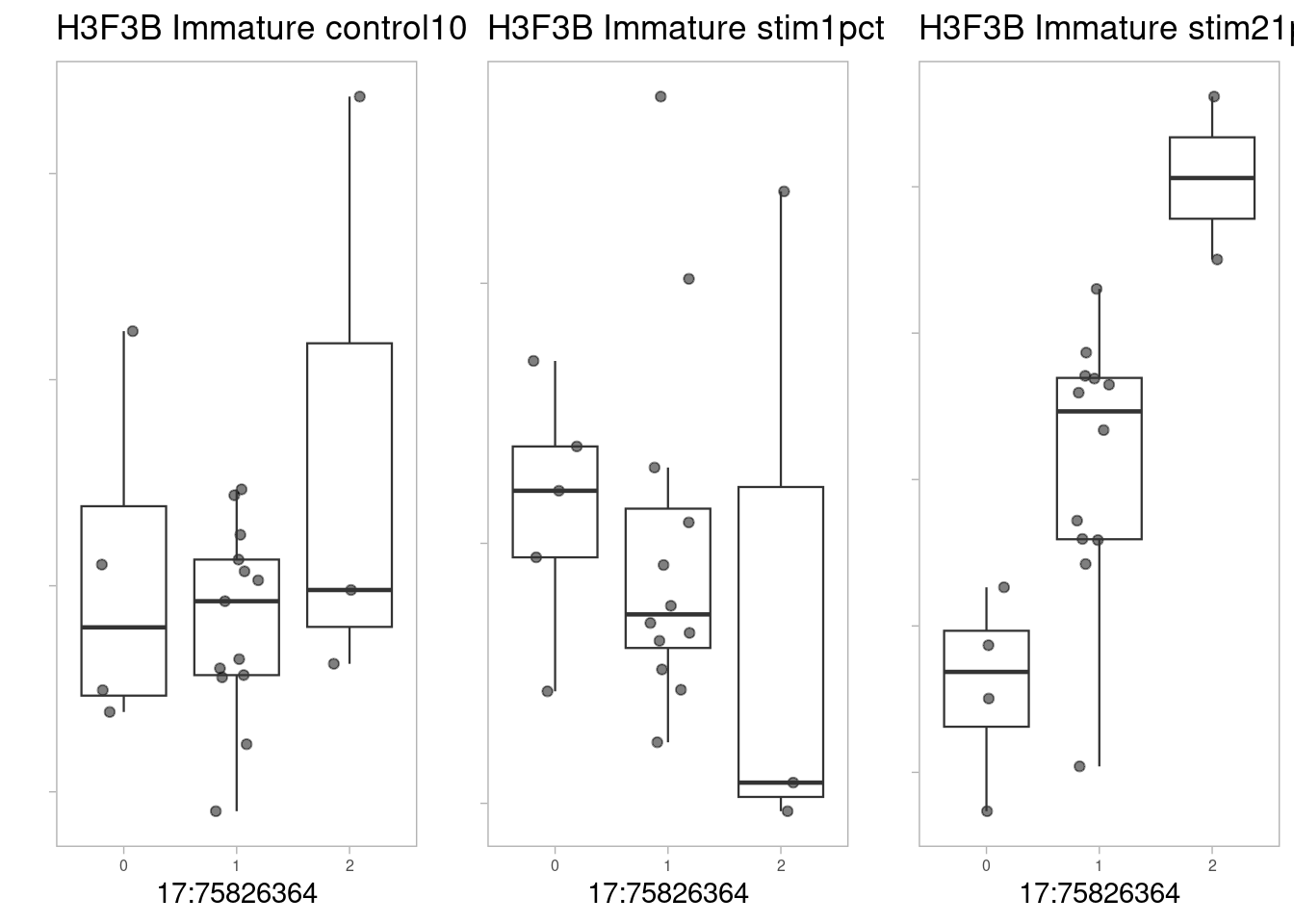
p1 <- make_boxplot(celltype = "IPcycling", condition = "control10", testsnp = "17:75826364", testgene = "H3F3B") + geom_boxplot(alpha=0, linewidth=0.4) + theme_classic() + theme(legend.position="none") + ylab("")+ theme(axis.text.x=element_text(size=6), axis.text.y=element_blank(), plot.background = element_blank(), panel.grid.major = element_blank(), panel.grid.minor = element_blank(), axis.title.y = element_blank())
── Column specification ────────────────────────────────────────────────────────
cols(
  ID = col_character(),
  NA19153 = col_double(),
  NA19207 = col_double(),
  NA18913 = col_double(),
  NA18853 = col_double(),
  NA18856 = col_double(),
  NA19093 = col_double(),
  NA19210 = col_double(),
  NA19190 = col_double(),
  NA18502 = col_double(),
  NA18517 = col_double(),
  NA18507 = col_double(),
  NA18501 = col_double(),
  NA18489 = col_double(),
  NA19102 = col_double(),
  NA19128 = col_double()
)
p2 <- make_boxplot(celltype = "IPcycling", condition = "stim1pct", testsnp = "17:75826364", testgene = "H3F3B") + geom_boxplot(alpha=0, linewidth=0.4) + theme_classic() + theme(legend.position="none") + ylab("")+ theme(axis.text.x=element_text(size=6), axis.text.y=element_blank(), plot.background = element_blank(), panel.grid.major = element_blank(), panel.grid.minor = element_blank(), axis.title.y = element_blank())
── Column specification ────────────────────────────────────────────────────────
cols(
  ID = col_character(),
  NA19153 = col_double(),
  NA19207 = col_double(),
  NA18913 = col_double(),
  NA18853 = col_double(),
  NA18856 = col_double(),
  NA19093 = col_double(),
  NA19144 = col_double(),
  NA19210 = col_double(),
  NA19190 = col_double(),
  NA18502 = col_double(),
  NA18517 = col_double(),
  NA18507 = col_double(),
  NA18501 = col_double(),
  NA18489 = col_double(),
  NA19102 = col_double(),
  NA19128 = col_double()
)
p3 <- make_boxplot(celltype = "IPcycling", condition = "stim21pct", testsnp = "17:75826364", testgene = "H3F3B") + geom_boxplot(alpha=0, linewidth=0.4) + theme_classic() + theme(legend.position="none") + ylab("")+ theme(axis.text.x=element_text(size=6), axis.text.y=element_blank(), plot.background = element_blank(), panel.grid.major = element_blank(), panel.grid.minor = element_blank(), axis.title.y = element_blank())
── Column specification ────────────────────────────────────────────────────────
cols(
  ID = col_character(),
  NA19153 = col_double(),
  NA19207 = col_double(),
  NA18913 = col_double(),
  NA18853 = col_double(),
  NA18856 = col_double(),
  NA19093 = col_double(),
  NA19210 = col_double(),
  NA19190 = col_double(),
  NA18502 = col_double(),
  NA18517 = col_double(),
  NA18507 = col_double(),
  NA18519 = col_double(),
  NA18501 = col_double(),
  NA18489 = col_double(),
  NA19102 = col_double(),
  NA19128 = col_double()
)
grid.arrange(p1, p2, p3, nrow=1)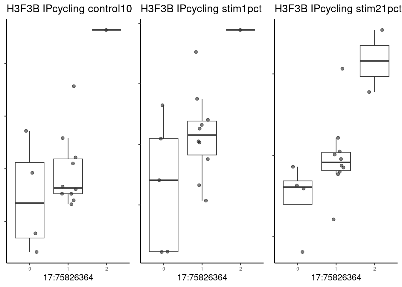
For the gene PPIA (cyclophilin A). Here, lfsr<0.2.
p1 <- make_boxplot(celltype = "NeuronOther", condition = "stim1pct", testsnp = "7:44768492", testgene = "PPIA") + geom_boxplot(alpha=0) + theme_classic() + theme(legend.position="none") + ylab("")
p2 <- make_boxplot(celltype = "NeuronOther", condition = "stim21pct", testsnp = "7:44768492", testgene = "PPIA") + geom_boxplot(alpha=0) + theme_classic() + theme(legend.position="none")+ ylab("")
p3 <- make_boxplot(celltype = "NeuronOther", condition = "control10", testsnp = "7:44768492", testgene = "PPIA") + geom_boxplot(alpha=0) + theme_classic() + theme(legend.position="none")+ ylab("")
grid.arrange(p3, p1, p2, nrow=1)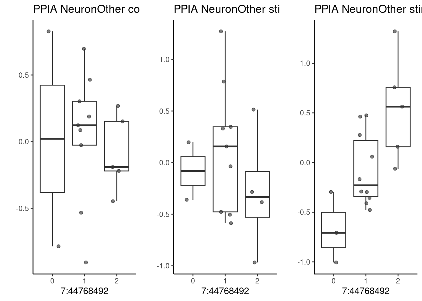
The following example genes do have significant effects in at least one condition (lfsr<0.1):
p1 <- make_boxplot(celltype = "Immature", condition = "stim1pct", testsnp = "14:103551768", testgene = "CKB") + geom_boxplot(alpha=0) + theme_classic() + theme(legend.position="none") + ylab("")
p2 <- make_boxplot(celltype = "Immature", condition = "stim21pct", testsnp = "14:103551768", testgene = "CKB") + geom_boxplot(alpha=0) + theme_classic() + theme(legend.position="none")+ ylab("")
p3 <- make_boxplot(celltype = "Immature", condition = "control10", testsnp = "14:103551768", testgene = "CKB") + geom_boxplot(alpha=0) + theme_classic() + theme(legend.position="none")+ ylab("")
grid.arrange(p3, p1, p2, nrow=1)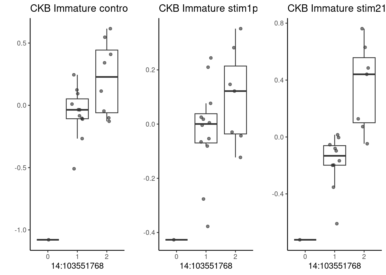
COA8, a cytochrome c oxidase interacting factor:
p1 <- make_boxplot(celltype = "InhThalamic", condition = "control10", testsnp = "14:103551768", testgene = "COA8") + geom_boxplot(alpha=0, linewidth=0.4) + theme_light() + theme(legend.position="none") + ylab("") +  theme(axis.text.x=element_text(size=6), axis.text.y=element_text(size=6), plot.background = element_blank(), panel.grid.major = element_blank(), panel.grid.minor = element_blank(), axis.title.y = element_blank())
p2 <- make_boxplot(celltype = "InhThalamic", condition = "stim1pct", testsnp = "14:103551768", testgene = "COA8") + geom_boxplot(alpha=0, linewidth=0.4) + theme_light() + theme(legend.position="none") + ylab("")+  theme(axis.text.x=element_text(size=6), axis.text.y=element_text(size=6), plot.background = element_blank(), panel.grid.major = element_blank(), panel.grid.minor = element_blank(), axis.title.y = element_blank())
p3 <- make_boxplot(celltype = "InhThalamic", condition = "stim21pct", testsnp = "14:103551768", testgene = "COA8") + geom_boxplot(alpha=0, linewidth=0.4) + theme_light() + theme(legend.position="none") + ylab("")+  theme(axis.text.x=element_text(size=6), axis.text.y=element_text(size=6), plot.background = element_blank(), panel.grid.major = element_blank(), panel.grid.minor = element_blank(), axis.title.y = element_blank())

grid.arrange(p1, p2, p3, nrow=1)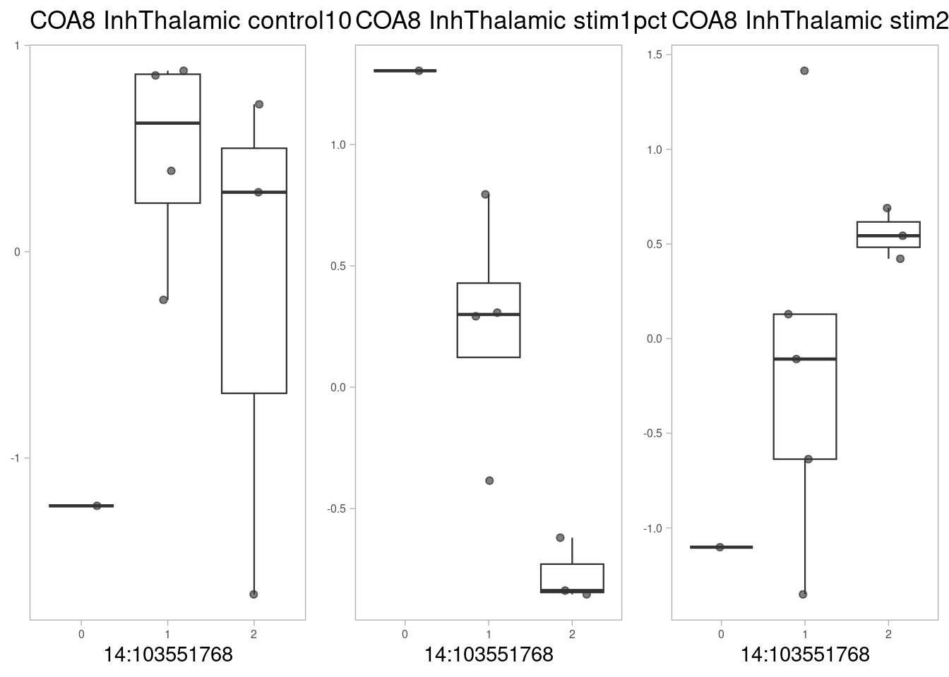
The gene RPS26, which has a significant QTL effect in multiple cell types. This SNP is associated with cognitive phenotypes.
p1 <- make_boxplot(celltype = "NeuronOther", condition = "stim1pct", testsnp = "12:56007301", testgene = "RPS26") + geom_boxplot(alpha=0) + theme_classic() + theme(legend.position="none") + ylab("")
── Column specification ────────────────────────────────────────────────────────
cols(
  ID = col_character(),
  NA19153 = col_double(),
  NA19207 = col_double(),
  NA18913 = col_double(),
  NA19098 = col_double(),
  NA19093 = col_double(),
  NA19144 = col_double(),
  NA19143 = col_double(),
  NA18502 = col_double(),
  NA18508 = col_double(),
  NA18517 = col_double(),
  NA18507 = col_double(),
  NA18501 = col_double(),
  NA18489 = col_double(),
  NA19102 = col_double(),
  NA18511 = col_double()
)
p2 <- make_boxplot(celltype = "NeuronOther", condition = "stim21pct", testsnp = "12:56007301", testgene = "RPS26") + geom_boxplot(alpha=0) + theme_classic() + theme(legend.position="none")+ ylab("")
── Column specification ────────────────────────────────────────────────────────
cols(
  ID = col_character(),
  NA19153 = col_double(),
  NA19207 = col_double(),
  NA18913 = col_double(),
  NA19098 = col_double(),
  NA18853 = col_double(),
  NA19093 = col_double(),
  NA19144 = col_double(),
  NA19143 = col_double(),
  NA19190 = col_double(),
  NA18502 = col_double(),
  NA18508 = col_double(),
  NA18517 = col_double(),
  NA18507 = col_double(),
  NA18501 = col_double(),
  NA18489 = col_double(),
  NA19102 = col_double(),
  NA18511 = col_double(),
  NA19128 = col_double()
)
p3 <- make_boxplot(celltype = "NeuronOther", condition = "control10", testsnp = "12:56007301", testgene = "RPS26") + geom_boxplot(alpha=0) + theme_classic() + theme(legend.position="none")+ ylab("")
── Column specification ────────────────────────────────────────────────────────
cols(
  ID = col_character(),
  NA19153 = col_double(),
  NA19207 = col_double(),
  NA18913 = col_double(),
  NA19098 = col_double(),
  NA18856 = col_double(),
  NA19093 = col_double(),
  NA19144 = col_double(),
  NA19143 = col_double(),
  NA18502 = col_double(),
  NA18508 = col_double(),
  NA18517 = col_double(),
  NA18507 = col_double(),
  NA18501 = col_double(),
  NA18489 = col_double(),
  NA19102 = col_double(),
  NA18511 = col_double()
)
grid.arrange(p3, p1, p2, nrow=1)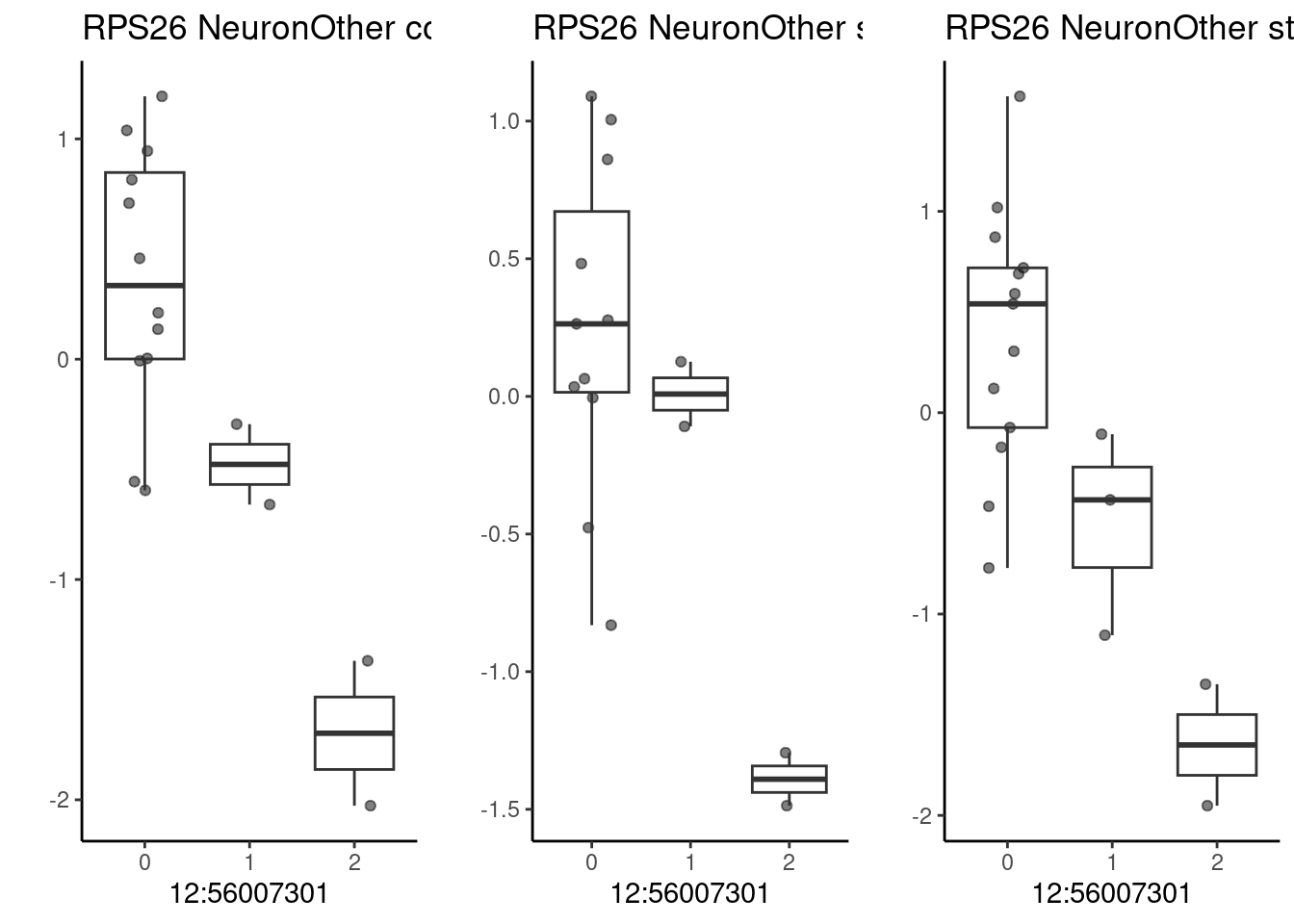
p1 <- make_boxplot(celltype = "RGcycling", condition = "stim1pct", testsnp = "12:56007301", testgene = "RPS26") + geom_boxplot(alpha=0) + theme_classic() + theme(legend.position="none") + ylab("")
p2 <- make_boxplot(celltype = "RGcycling", condition = "stim21pct", testsnp = "12:56007301", testgene = "RPS26") + geom_boxplot(alpha=0) + theme_classic() + theme(legend.position="none")+ ylab("")
p3 <- make_boxplot(celltype = "RGcycling", condition = "control10", testsnp = "12:56007301", testgene = "RPS26") + geom_boxplot(alpha=0) + theme_classic() + theme(legend.position="none")+ ylab("")
grid.arrange(p3, p1, p2, nrow=1)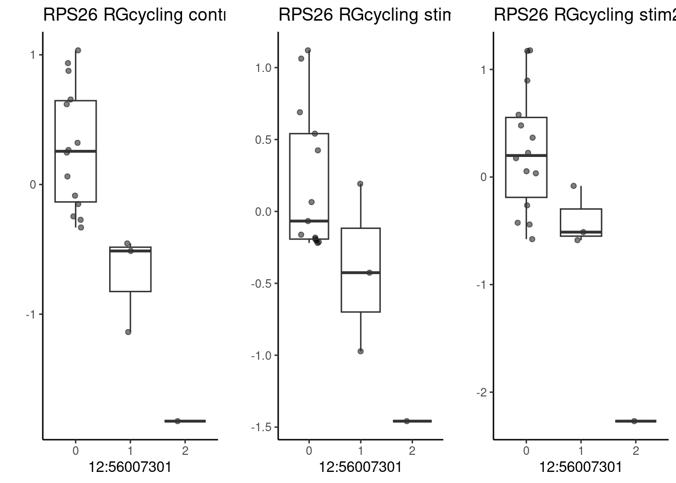
p1 <- make_boxplot(celltype = "GliaProg", condition = "stim1pct", testsnp = "12:56007301", testgene = "RPS26") + geom_boxplot(alpha=0) + theme_classic() + theme(legend.position="none") + ylab("")
p2 <- make_boxplot(celltype = "GliaProg", condition = "stim21pct", testsnp = "12:56007301", testgene = "RPS26") + geom_boxplot(alpha=0) + theme_classic() + theme(legend.position="none")+ ylab("")
p3 <- make_boxplot(celltype = "GliaProg", condition = "control10", testsnp = "12:56007301", testgene = "RPS26") + geom_boxplot(alpha=0) + theme_classic() + theme(legend.position="none")+ ylab("")
grid.arrange(p3, p1, p2, nrow=1)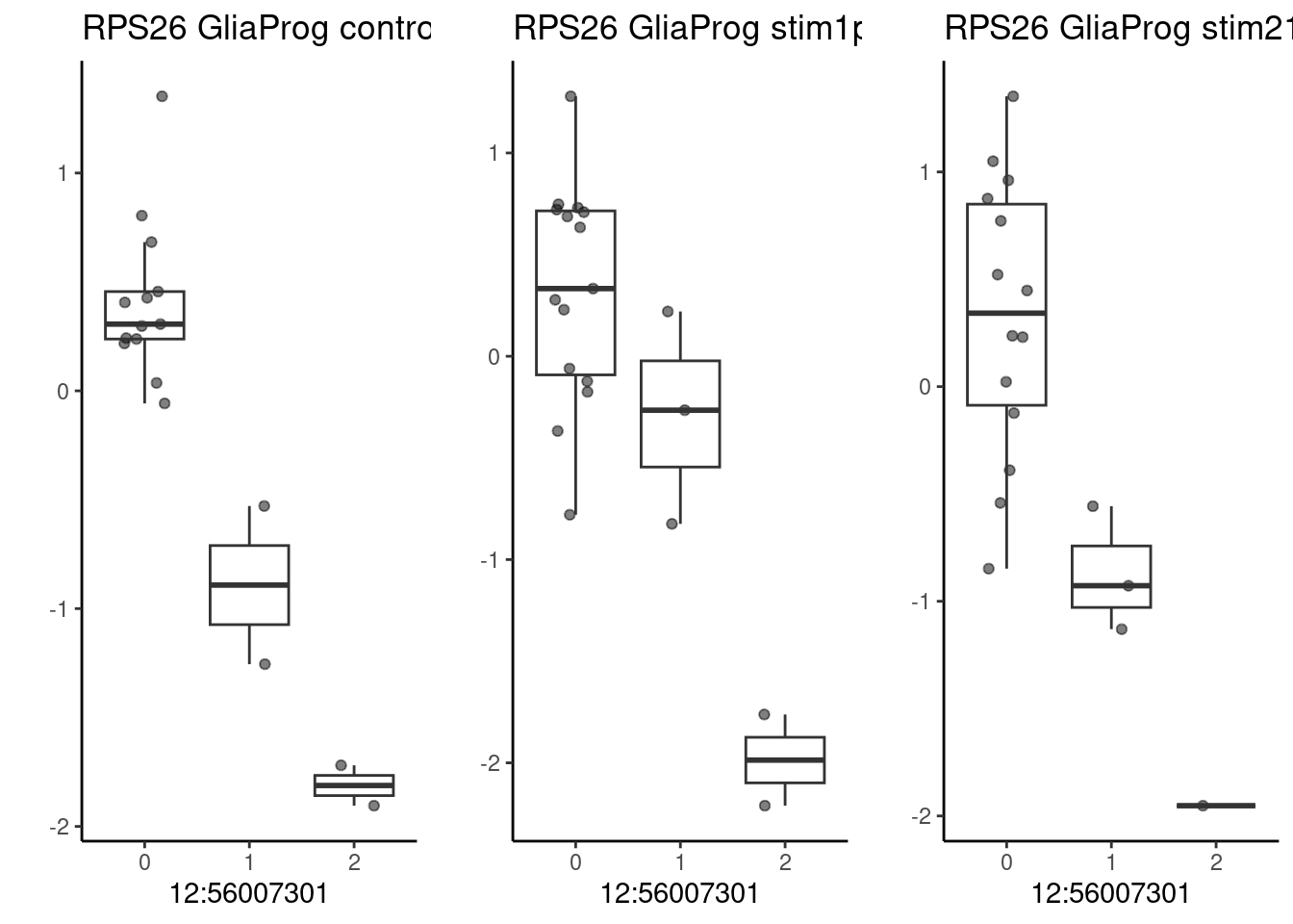
And PLRG1, an important and pleiotropic regulator, which has a significant eQTL effect only under normoxia that is suppressed under oxygen stress. This SNP is strongly associated with stroke risk (GCST005838, GCST005843).
p1 <- make_boxplot(celltype = "CorticalHem", condition = "stim1pct", testsnp = "4:154580036", testgene = "PLRG1") + geom_boxplot(alpha=0) + theme_classic() + theme(legend.position="none") + ylab("")
p2 <- make_boxplot(celltype = "CorticalHem", condition = "stim21pct", testsnp = "4:154580036", testgene = "PLRG1") + geom_boxplot(alpha=0) + theme_classic() + theme(legend.position="none")+ ylab("")
p3 <- make_boxplot(celltype = "CorticalHem", condition = "control10", testsnp = "4:154580036", testgene = "PLRG1") + geom_boxplot(alpha=0) + theme_classic() + theme(legend.position="none")+ ylab("")
grid.arrange(p3, p1, p2, nrow=1)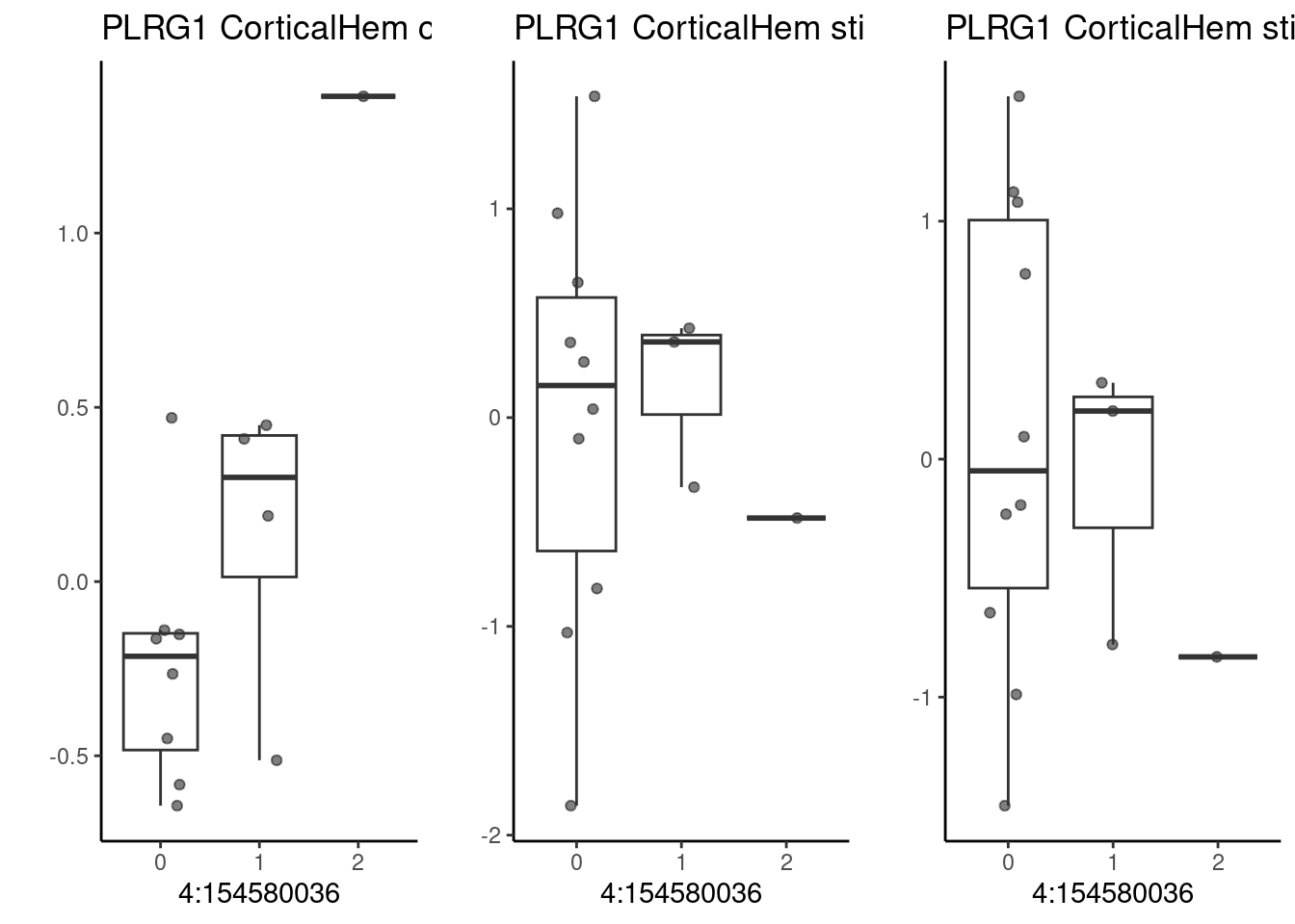
sessionInfo()R version 4.2.0 (2022-04-22)
Platform: x86_64-pc-linux-gnu (64-bit)
Running under: CentOS Linux 7 (Core)
Matrix products: default
BLAS/LAPACK: /software/openblas-0.3.13-el7-x86_64/lib/libopenblas_haswellp-r0.3.13.so
locale:
[1] LC_CTYPE=en_US.UTF-8 LC_NUMERIC=C LC_TIME=C
[4] LC_COLLATE=C LC_MONETARY=C LC_MESSAGES=C
[7] LC_PAPER=C LC_NAME=C LC_ADDRESS=C
[10] LC_TELEPHONE=C LC_MEASUREMENT=C LC_IDENTIFICATION=C
attached base packages:
[1] stats4 stats graphics grDevices utils datasets methods
[8] base
other attached packages:
[1] GenomicRanges_1.50.2 GenomeInfoDb_1.34.9 IRanges_2.32.0
[4] S4Vectors_0.36.2 BiocGenerics_0.44.0 vroom_1.6.4
[7] MatrixEQTL_2.3 gridExtra_2.3 ggrepel_0.9.4
[10] knitr_1.45 udr_0.3-153 mashr_0.2.79
[13] ashr_2.2-63 RColorBrewer_1.1-3 pals_1.8
[16] lubridate_1.9.3 forcats_1.0.0 stringr_1.5.0
[19] dplyr_1.1.4 purrr_1.0.2 readr_2.1.4
[22] tidyr_1.3.0 tibble_3.2.1 ggplot2_3.4.4
[25] tidyverse_2.0.0 SeuratObject_4.1.4 Seurat_4.4.0
[28] workflowr_1.7.0
loaded via a namespace (and not attached):
[1] plyr_1.8.9 igraph_1.5.1 lazyeval_0.2.2
[4] sp_2.1-3 splines_4.2.0 listenv_0.9.1
[7] scattermore_1.2 digest_0.6.34 invgamma_1.1
[10] htmltools_0.5.7 SQUAREM_2021.1 fansi_1.0.5
[13] magrittr_2.0.3 tensor_1.5 cluster_2.1.3
[16] ROCR_1.0-11 tzdb_0.4.0 globals_0.16.2
[19] matrixStats_1.1.0 timechange_0.2.0 spatstat.sparse_3.0-3
[22] colorspace_2.1-0 xfun_0.41 RCurl_1.98-1.13
[25] crayon_1.5.2 callr_3.7.3 jsonlite_1.8.7
[28] progressr_0.14.0 spatstat.data_3.0-3 survival_3.3-1
[31] zoo_1.8-12 glue_1.6.2 polyclip_1.10-0
[34] gtable_0.3.4 zlibbioc_1.44.0 XVector_0.38.0
[37] leiden_0.4.2 future.apply_1.11.1 maps_3.4.0
[40] abind_1.4-5 scales_1.2.1 mvtnorm_1.2-3
[43] spatstat.random_3.1-3 miniUI_0.1.1.1 Rcpp_1.0.12
[46] viridisLite_0.4.2 xtable_1.8-4 reticulate_1.34.0
[49] bit_4.0.5 mapproj_1.2.11 truncnorm_1.0-9
[52] htmlwidgets_1.6.2 httr_1.4.7 ellipsis_0.3.2
[55] ica_1.0-3 farver_2.1.1 pkgconfig_2.0.3
[58] sass_0.4.7 uwot_0.1.16 deldir_1.0-6
[61] utf8_1.2.4 labeling_0.4.3 tidyselect_1.2.0
[64] rlang_1.1.3 reshape2_1.4.4 later_1.3.0
[67] munsell_0.5.0 tools_4.2.0 cachem_1.0.8
[70] cli_3.6.1 generics_0.1.3 ggridges_0.5.3
[73] evaluate_0.23 fastmap_1.1.1 yaml_2.3.5
[76] goftest_1.2-3 bit64_4.0.5 processx_3.8.2
[79] fs_1.6.3 fitdistrplus_1.1-8 RANN_2.6.1
[82] pbapply_1.5-0 future_1.33.1 nlme_3.1-157
[85] whisker_0.4.1 mime_0.12 compiler_4.2.0
[88] rstudioapi_0.17.1 plotly_4.10.0 png_0.1-8
[91] spatstat.utils_3.0-4 bslib_0.5.1 stringi_1.8.1
[94] highr_0.9 ps_1.7.5 lattice_0.20-45
[97] Matrix_1.6-3 vctrs_0.6.4 pillar_1.9.0
[100] lifecycle_1.0.4 spatstat.geom_3.2-7 lmtest_0.9-40
[103] jquerylib_0.1.4 RcppAnnoy_0.0.19 bitops_1.0-7
[106] data.table_1.14.8 cowplot_1.1.1 irlba_2.3.5.1
[109] httpuv_1.6.5 patchwork_1.1.3 R6_2.5.1
[112] promises_1.2.0.1 KernSmooth_2.23-20 parallelly_1.37.0
[115] codetools_0.2-18 dichromat_2.0-0.1 assertthat_0.2.1
[118] MASS_7.3-56 rprojroot_2.0.3 withr_2.5.2
[121] sctransform_0.4.1 GenomeInfoDbData_1.2.9 parallel_4.2.0
[124] hms_1.1.3 grid_4.2.0 rmarkdown_2.26
[127] Rtsne_0.16 git2r_0.30.1 mixsqp_0.3-48
[130] getPass_0.2-2 spatstat.explore_3.0-6 shiny_1.7.5.1
[133] rmeta_3.0