figure3

workflowr

• Summary
• Checks
• Past versions

Last updated: 2025-04-19

Checks: 7 0

Knit directory: organoid_oxygen_eqtl/

This reproducible R Markdown analysis was created with workflowr (version 1.7.0). The Checks tab describes the reproducibility checks that were applied when the results were created. The Past versions tab lists the development history.

---

R Markdown file: up-to-date

Great! Since the R Markdown file has been committed to the Git repository, you know the exact version of the code that produced these results.

Environment: empty

Great job! The global environment was empty. Objects defined in the global environment can affect the analysis in your R Markdown file in unknown ways. For reproduciblity it’s best to always run the code in an empty environment.

Seed: set.seed(20250224)

The command set.seed(20250224) was run prior to running the code in the R Markdown file. Setting a seed ensures that any results that rely on randomness, e.g. subsampling or permutations, are reproducible.

Session information: recorded

Great job! Recording the operating system, R version, and package versions is critical for reproducibility.

Cache: none

Nice! There were no cached chunks for this analysis, so you can be confident that you successfully produced the results during this run.

File paths: relative

Great job! Using relative paths to the files within your workflowr project makes it easier to run your code on other machines.

Repository version: 03481ab

Great! You are using Git for version control. Tracking code development and connecting the code version to the results is critical for reproducibility.

The results in this page were generated with repository version 03481ab. See the Past versions tab to see a history of the changes made to the R Markdown and HTML files.

Note that you need to be careful to ensure that all relevant files for the analysis have been committed to Git prior to generating the results (you can use wflow_publish or wflow_git_commit). workflowr only checks the R Markdown file, but you know if there are other scripts or data files that it depends on. Below is the status of the Git repository when the results were generated:

Ignored files:
    Ignored:    .DS_Store
    Ignored:    analysis/.Rhistory
    Ignored:    analysis/figure/
    Ignored:    code/.DS_Store

Unstaged changes:
    Deleted:    code/mash_EE.R
    Modified:   code/mash_EE_PC.R

Note that any generated files, e.g. HTML, png, CSS, etc., are not included in this status report because it is ok for generated content to have uncommitted changes.

---

These are the previous versions of the repository in which changes were made to the R Markdown (analysis/figure3.Rmd) and HTML (docs/figure3.html) files. If you’ve configured a remote Git repository (see ?wflow_git_remote), click on the hyperlinks in the table below to view the files as they were in that past version.

File	Version	Author	Date	Message
Rmd	03481ab	Ben Umans	2025-04-19	updated April 2025
html	d3c2181	Ben Umans	2025-02-25	Build site.
Rmd	e2e7046	Ben Umans	2025-02-25	updated plot formatting
html	f357871	Ben Umans	2025-02-24	Build site.
Rmd	3b3a54d	Ben Umans	2025-02-24	updated mash SE and compile for resubmission
Rmd	f0eaf05	Ben Umans	2024-09-05	organized for upload to github
html	f0eaf05	Ben Umans	2024-09-05	organized for upload to github

---

Introduction

This page describes steps used to map eQTLs, fit a topic model, and map topic-interacting eQTLs, corresponding to Figure 3.

library(Seurat)

Attaching SeuratObject

library(tidyverse)

── Attaching core tidyverse packages ──────────────────────── tidyverse 2.0.0 ──
✔ dplyr     1.1.4     ✔ readr     2.1.4
✔ forcats   1.0.0     ✔ stringr   1.5.0
✔ ggplot2   3.4.4     ✔ tibble    3.2.1
✔ lubridate 1.9.3     ✔ tidyr     1.3.0
✔ purrr     1.0.2     

── Conflicts ────────────────────────────────────────── tidyverse_conflicts() ──
✖ dplyr::filter() masks stats::filter()
✖ dplyr::lag()    masks stats::lag()
ℹ Use the conflicted package (<http://conflicted.r-lib.org/>) to force all conflicts to become errors

library(pals)
library(RColorBrewer)
library(pheatmap)
library(magrittr)

Attaching package: 'magrittr'

The following object is masked from 'package:purrr':

    set_names

The following object is masked from 'package:tidyr':

    extract

library(ggpointdensity)
library(viridis)

Loading required package: viridisLite

Attaching package: 'viridisLite'

The following objects are masked from 'package:pals':

    cividis, inferno, magma, plasma, turbo, viridis


Attaching package: 'viridis'

The following objects are masked from 'package:pals':

    cividis, inferno, magma, plasma, turbo, viridis

library(mashr)

Loading required package: ashr

library(udr)
library(ggrepel)
library(pheatmap)
library(MatrixEQTL)
library(qvalue)
library(snpStats)

Loading required package: survival
Loading required package: Matrix

Attaching package: 'Matrix'

The following objects are masked from 'package:tidyr':

    expand, pack, unpack

library(gdata)

Attaching package: 'gdata'

The following objects are masked from 'package:dplyr':

    combine, first, last

The following object is masked from 'package:purrr':

    keep

The following object is masked from 'package:stats':

    nobs

The following object is masked from 'package:utils':

    object.size

The following object is masked from 'package:base':

    startsWith

library(vroom)

Attaching package: 'vroom'

The following objects are masked from 'package:readr':

    as.col_spec, col_character, col_date, col_datetime, col_double,
    col_factor, col_guess, col_integer, col_logical, col_number,
    col_skip, col_time, cols, cols_condense, cols_only, date_names,
    date_names_lang, date_names_langs, default_locale, fwf_cols,
    fwf_empty, fwf_positions, fwf_widths, locale, output_column,
    problems, spec

library(ggblend)
source("analysis/shared_functions_style_items.R")

eQTL identification using MatrixEQTL

Mapping eQTLs using MatrixEQTL requires the following inputs: * SNP names * SNP locations * gene locations * expression phenotypes * covariates * error covariance (relatedness) + estimated relatedness matrix from Gemma showed all individuals in our dataset were equally unrelated; we therefore did not include kinship information in the model

SNP names and locations

First, use vcftools to filter the genotype VCF to only the cell lines included in this data collection. Further filter loci by HWE, minor allele frequency, and maximum number alleles, splitting by chromosome.

module load vcftools
for g in /project/gilad/1KG_HighCoverageCalls2021/*vcf.gz;
do
q="$(basename -- $g)"
vcftools --gzvcf $g --keep MatrixEQTL/sample_list --maf 0.1 --max-alleles 2 --max-missing 1 --hwe 0.000001 --remove-indels --recode --out MatrixEQTL/snps/YRI_genotypes_maf10hwee-6_full/${q}
done

Next, I used bcftools to reformat the output according to MatrixEQTL’s input requirements:

for g in MatrixEQTL/snps/YRI_genotypes_maf10hwee-6_full/*recode.vcf
do
bcftools query -f '%ID[\t%GT]\n' ${g} > ${g}.snps;
bcftools query -f '%ID\t%CHROM\t%POS\n' ${g} > ${g}.snploc
done

Next, replace genotypes with allele counts, meaning 0/0 becomes 0, 0/1 becomes 1, and 1/1 becomes 2.

For the single chromosome:

for i in *.snps
do
sed -i 's:1/1:2:g' ${i}; sed -i 's:0/1:1:g' ${i}; sed -i 's:1/0:1:g' ${i}; sed -i 's:0/0:0:g' ${i}
done

for i in *.snps
do
sed -i 's:1|1:2:g' ${i}; sed -i 's:0|1:1:g' ${i}; sed -i 's:1|0:1:g' ${i}; sed -i 's:0|0:0:g' ${i}
done

Finally, add back the cell line names (obtained from bcftools view -h) to name the columns, which was lost in the bcftools query operation.

for i in *.snps
do
chromname=`basename $i .snps`;
cat ../SNP_header ${chromname}.snps > ${chromname}_for_matrixeqtl.snps;
cat ../SNPloc_header ${chromname}.snploc > ${chromname}_for_matrixeqtl.snploc
done

Gene locations

We mapped eQTLs within 50 kb of each gene’s TSS, treating each chromosome independently.

for(d in 1:22){
  TSSlocs <- read.table("/project2/gilad/kenneth/References/human/cellranger/cellranger4.0/refdata-gex-GRCh38-2020-A/genes/genes.ucsc.sorted.bed", header=F) %>% 
  filter(V9=="protein_coding" | V9=="lncRNA" | V9=="pseudogene") %>% 
  group_by(V8) %>% 
  summarise(chr=V1[1], start=if_else(V6[1]=="+", min(V2), max(V3)), end=if_else(V6[1]=="+", min(V2)+1, max(V3)+1), gene=V8[1]) %>% 
  select(gene, chr, start, end) %>% 
    filter(chr==paste("chr", d, sep = "")) %>% 
  arrange(chr, start) 
write.table(TSSlocs, file = paste("data/MatrixEQTL/snps/TSSlocs_chr", d, ".locs", sep=""), row.names = F, col.names = T, quote=F, sep = "\t")
}

Gene expression

The following function takes pseudobulk input to writes out formatted, normalized data for MatrixEQTL.

makeExprTableMatrixEQTL_byChr <- function(pseudo, outdir, outprefix, pseudo.classifications, transcriptome, min.count.cpm=0, min.prop.expr=0.5, min.total.count=30) {
  for (k in unlist(unique(pseudo$meta[[pseudo.classifications[1]]]))){
    for (j in unlist(unique(pseudo$meta[[pseudo.classifications[2]]]))){
      counts <- as.matrix(pseudo$counts[, which(pseudo$meta[[pseudo.classifications[1]]]==k & pseudo$meta[[pseudo.classifications[2]]]==j)])
      print(paste0(ncol(counts), " samples retained for ", k, " and ", j))
      if (ncol(counts) < 3){
        next
      }
      DEG <- DGEList(counts = as.matrix(counts))
      keep <- filterByExpr(y = DEG, min.count = min.count.cpm, 
                           min.prop=min.prop.expr, 
                           min.total.count = min.total.count)
      print(paste0("Retained ", sum(keep), " genes"))

      DEG <- DEG[keep, , keep.lib.sizes=FALSE]
      keep <- rowSds(cpm(DEG))>summary(rowSds(cpm(DEG)))[2]
      DEG <- DEG[keep, , keep.lib.sizes=FALSE]
      DEG <- calcNormFactors(DEG, method="TMM")
      
      DEG_cpm <- edgeR::cpm(DEG, log = TRUE)
      colnames(DEG_cpm) <- as.factor(str_sub(colnames(DEG_cpm), start = -7))
      DEG_cpm <- data.frame(DEG_cpm)
      
     DEG_inorm <- DEG_cpm %>% 
       rownames_to_column("ID") %>%
       gather("SampleName", "value", -ID) %>% 
       dplyr::group_by(ID) %>% 
       dplyr::mutate(scaled_values = scale_this(value)) %>% 
       dplyr::ungroup() %>% 
       dplyr::group_by(SampleName) %>%
       dplyr::mutate(scaled_value_percentiles = rank(scaled_values, ties.method = "average")/(n()+1)) %>%
       dplyr::mutate(ScaledAndInverseNormalized = qnorm(scaled_value_percentiles)) %>%
       ungroup() %>% 
       dplyr::select(ID, SampleName, ScaledAndInverseNormalized) %>% 
       pivot_wider(names_from="SampleName", values_from="ScaledAndInverseNormalized") %>%
       dplyr::select(ID, everything()) 
 
      for (q in 1:22){
        geneset <- filter(transcriptome, `#chr`==paste("chr", q, sep=""))$id
        DEG_inorm_write <- DEG_inorm %>% filter(ID %in% geneset)
        write.table(DEG_inorm_write, file = paste(outdir, "expressiontable_matrixeqtl_", outprefix, k, "_" , j, "_chr", q, "_cpm-inorm.bed", sep=""), row.names = F, col.names = T, quote=F, sep = "\t")
        }
      }
      rm(DEG, DEG_cpm, keep, counts, DEG_inorm)
    }
  }

I format the transcriptome and filter to protein coding genes:

transcriptome <- read.table("/project2/gilad/kenneth/References/human/cellranger/cellranger4.0/refdata-gex-GRCh38-2020-A/genes/genes.ucsc.sorted.bed", header=F) %>% 
  filter(V9=="protein_coding") %>% 
  group_by(V8) %>% 
  dplyr::summarise(chr=V1[1], start=if_else(V6[1]=="+", min(V2), max(V3)), end=if_else(V6[1]=="+", min(V2)+1, max(V3)+1), id=V8[1]) %>% 
  select(chr, start, end, id) %>% 
  arrange(chr, start) %>% 
  dplyr::summarise("#chr"=chr, start=start, end=end, id=id)

Warning: Returning more (or less) than 1 row per `summarise()` group was deprecated in
dplyr 1.1.0.
ℹ Please use `reframe()` instead.
ℹ When switching from `summarise()` to `reframe()`, remember that `reframe()`
  always returns an ungrouped data frame and adjust accordingly.
Call `lifecycle::last_lifecycle_warnings()` to see where this warning was
generated.

Then pseudobulk and process the expression data:

subset_seurat <- subset(harmony.batchandindividual.sct, subset = vireo.prob.singlet > 0.95 & nCount_RNA<20000 & nCount_RNA>2500 )

pseudo_coarse_quality <- generate.pseudobulk(subset_seurat, labels = c("combined.annotation.coarse.harmony", "treatment", "vireo.individual"))

pseudo_fine_quality <- generate.pseudobulk(subset_seurat, labels = c("combined.annotation.fine.harmony", "treatment", "vireo.individual"))

pseudo_coarse_quality <- filter.pseudobulk(pseudo_coarse_quality, threshold = 20)

makeExprTableMatrixEQTL_byChr(pseudo = pseudo_coarse_quality, outdir = "/project2/gilad/umans/oxygen_eqtl/data/MatrixEQTL/expression/combined_coarse_quality_filter20_032024/", outprefix = "combined_coarse_", pseudo.classifications = c("treatment", "combined.annotation.coarse.harmony"), transcriptome = transcriptome, min.count.cpm=6, min.prop.expr=0.5, min.total.count=30)


pseudo_fine_quality <- filter.pseudobulk(pseudo_fine_quality, threshold = 20)

makeExprTableMatrixEQTL_byChr(pseudo = pseudo_fine_quality, outdir = "/project2/gilad/umans/oxygen_eqtl/data/MatrixEQTL/expression/combined_fine_quality_filter20_032024/", outprefix = "combined_fine_", pseudo.classifications = c("treatment", "combined.annotation.fine.harmony"), transcriptome = transcriptome, min.count.cpm=6, min.prop.expr=0.5, min.total.count=30)

Covariates

EQTLs were estimated with a model that included expression principal components as covariates. The number of expression PCs was chosen so as to explain more variation in the observed data than in a random permutation of the expression values.
This was done in the same way for the coarsely- and finely-clustered data:

for (condition in c("control10", "stim1pct", "stim21pct")){
  for (celltype in c("Cajal", "Choroid",  "Glia", "Glut", "Immature", "IP", "Inh", "RG", "NeuronOther", "VLMC")){
    pheno <- data.frame(t(read.table(paste0("data/MatrixEQTL/expression/combined_coarse_quality_filter20_032024/expressiontable_matrixeqtl_combined_coarse_", condition, "_", celltype, "_chr1_cpm-inorm.bed"), header = TRUE)[,-1])) %>% rownames_to_column(var="individual") %>% arrange(individual) %>% column_to_rownames(var="individual") %>% as.matrix()
    for (chrom in 2:22){
      cbind(pheno, data.frame(t(read.table(paste0("data/MatrixEQTL/expression/combined_coarse_quality_filter20_032024/expressiontable_matrixeqtl_combined_coarse_", condition, "_", celltype, "_chr", chrom, "_cpm-inorm.bed"), header = TRUE)[,-1])) %>% rownames_to_column(var="individual") %>% arrange(individual) %>% column_to_rownames(var="individual") %>% as.matrix())
    }
    
     pheno.permuted <- matrix(nrow=nrow(pheno), ncol=ncol(pheno))
  for (i in 1:nrow(pheno)){
     pheno.permuted[i,] <- sample(pheno[i,], size=ncol(pheno))
  }
  pca.results <- prcomp(pheno)
    
  pca <- pca.results %>% summary() %>% extract2("importance") %>% 
    t() %>% 
    as.data.frame() %>%
    rownames_to_column("PC")
  pca.permuted <- prcomp(pheno.permuted) %>% summary() %>% extract2("importance") %>% t() %>% as.data.frame() %>% rownames_to_column("PC")
  
  merged <- bind_rows(list(pca=pca, pca.permuted=pca.permuted), .id="source") %>%
        mutate(PC=as.numeric(str_replace(PC, "PC", "")))
    
    #Get number of PCs
  NumPCs <- merged %>%
      dplyr::select(PC, Prop=`Proportion of Variance`, source) %>%
      spread(key="source", value="Prop") %>%
      filter(pca > pca.permuted) %>% pull(PC) %>% max()
    
  if (NumPCs >= nrow(pheno)){
    NumPCs <- nrow(pheno) - 1
  }
  for (outchrom in 1:22){
    pca.results$x[,1:NumPCs] %>% t() %>%
      round(5) %>%
      as.data.frame() %>%
      rownames_to_column("id") %>% 
      write_tsv(paste0("data/MatrixEQTL/covariates/combined_coarse_quality_filter20_032024/expressiontable_matrixeqtl_combined_coarse_", condition, "_", celltype, "_chr", outchrom, "_cpm-inorm.bed.covs"))
  }
  print(paste0(celltype, " done!", "\n"))
  rm(pheno, pheno.permuted, pca.results, NumPCs, merged)
  }
}

For finely clustered:

for (condition in c("control10", "stim1pct", "stim21pct")){
  for (celltype in c("Cajal", "Choroid", "CorticalHem", "GliaProg", "Glut", "GlutNTS", "Immature", "IP", "IPcycling", "Inh", "InhGNRH", "InhThalamic", "InhSST", "RG", "RGcycling", "NeuronOther", "VLMC")){
    pheno <- data.frame(t(read.table(paste0("data/MatrixEQTL/expression/combined_fine_quality_filter20_032024/expressiontable_matrixeqtl_combined_fine_", condition, "_", celltype, "_chr1_cpm-inorm.bed"), header = TRUE)[,-1])) %>% rownames_to_column(var="individual") %>% arrange(individual) %>% column_to_rownames(var="individual") %>% as.matrix()
    for (chrom in 2:22){
      cbind(pheno, data.frame(t(read.table(paste0("data/MatrixEQTL/expression/combined_fine_quality_filter20_032024/expressiontable_matrixeqtl_combined_fine_", condition, "_", celltype, "_chr", chrom, "_cpm-inorm.bed"), header = TRUE)[,-1])) %>% rownames_to_column(var="individual") %>% arrange(individual) %>% column_to_rownames(var="individual") %>% as.matrix())
    }
  
  pheno.permuted <- matrix(nrow=nrow(pheno), ncol=ncol(pheno))
  for (i in 1:nrow(pheno)){
     pheno.permuted[i,] <- sample(pheno[i,], size=ncol(pheno))
  }
  pca.results <- prcomp(pheno)
  
  pca <- pca.results %>% summary() %>% extract2("importance") %>% t() %>% as.data.frame() %>%
    rownames_to_column("PC")
  pca.permuted <- prcomp(pheno.permuted) %>% summary() %>% extract2("importance") %>% t() %>% as.data.frame() %>% rownames_to_column("PC")
  
  merged <- bind_rows(list(pca=pca, pca.permuted=pca.permuted), .id="source") %>%
      mutate(PC=as.numeric(str_replace(PC, "PC", "")))
  
  #Get number of PCs
  NumPCs <- merged %>%
      dplyr::select(PC, Prop=`Proportion of Variance`, source) %>%
      spread(key="source", value="Prop") %>%
      filter(pca > pca.permuted) %>% pull(PC) %>% max()

  if (NumPCs >= nrow(pheno)){
    NumPCs <- nrow(pheno) - 1
  }
  
  for (outchrom in 1:22){
    pca.results$x[,1:NumPCs] %>% t() %>%
      round(5) %>%
      as.data.frame() %>%
      rownames_to_column("id") %>% 
      write_tsv(paste0("data/MatrixEQTL/covariates/combined_fine_quality_filter20_032024/expressiontable_matrixeqtl_combined_fine_", condition, "_", celltype, "_chr", outchrom, "_cpm-inorm.bed.covs"))
  }
 
  print(paste0(celltype, " done!", "\n"))
   rm(pheno, pheno.permuted, pca.results, NumPCs, merged)
  }
}

Going forward, we omit the following cell types, which have too few individuals in one condition and, consequently, produce unstable covariate estimates: Cajal-Retzius cells, SST+ inhibitory neurons, VLMC.

MatrixEQTL and mash processing of results

Now I run MatrixEQTL in each cell type and each condition, using shell script MatrixEQTL_simple.sh.

module load R/4.2.0
for celltype in Glia Glut Immature IP Inh NeuronOther RG ; 
do
sh MatrixEQTL_simple.sh  /project2/gilad/umans/oxygen_eqtl/data/MatrixEQTL "combined_coarse_quality_filter20_032024/expressiontable_matrixeqtl_combined_coarse_control10" "YRI_genotypes_maf10hwee-6_full" /project2/gilad/umans/oxygen_eqtl/data/MatrixEQTL/snps/TSSlocs.locs  /project2/gilad/umans/oxygen_eqtl/data/relatedness/YRI_relatedness_gemma.sXX.txt 50000 2 ${celltype}
sleep 0.1
done

for celltype in Glia Glut Immature IP Inh NeuronOther RG ; 
do
sh MatrixEQTL_simple.sh  /project2/gilad/umans/oxygen_eqtl/data/MatrixEQTL "combined_coarse_quality_filter20_032024/expressiontable_matrixeqtl_combined_coarse_stim1pct" "YRI_genotypes_maf10hwee-6_full" /project2/gilad/umans/oxygen_eqtl/data/MatrixEQTL/snps/TSSlocs.locs  /project2/gilad/umans/oxygen_eqtl/data/relatedness/YRI_relatedness_gemma.sXX.txt 50000 2 ${celltype}
sleep 0.1
done
for celltype in Glia Glut Immature IP Inh NeuronOther RG ; 
do
sh MatrixEQTL_simple.sh  /project2/gilad/umans/oxygen_eqtl/data/MatrixEQTL "combined_coarse_quality_filter20_032024/expressiontable_matrixeqtl_combined_coarse_stim21pct" "YRI_genotypes_maf10hwee-6_full" /project2/gilad/umans/oxygen_eqtl/data/MatrixEQTL/snps/TSSlocs.locs  /project2/gilad/umans/oxygen_eqtl/data/relatedness/YRI_relatedness_gemma.sXX.txt 50000 2 ${celltype}
sleep 0.1
done

module load R/4.2.0
for celltype in CorticalHem GliaProg Glut GlutNTS Immature IP IPcycling Inh InhGNRH  InhThalamic RG RGcycling NeuronOther ;
do
sh MatrixEQTL_simple.sh  /project2/gilad/umans/oxygen_eqtl/data/MatrixEQTL "combined_fine_quality_filter20_032024/expressiontable_matrixeqtl_combined_fine_control10" "YRI_genotypes_maf10hwee-6_full" /project2/gilad/umans/oxygen_eqtl/data/MatrixEQTL/snps/TSSlocs.locs  /project2/gilad/umans/oxygen_eqtl/data/relatedness/YRI_relatedness_gemma.sXX.txt 50000 2 ${celltype}
sleep 0.1
done

for celltype in CorticalHem GliaProg Glut GlutNTS Immature IP IPcycling Inh InhGNRH  InhThalamic RG RGcycling NeuronOther ;
do
sh MatrixEQTL_simple.sh  /project2/gilad/umans/oxygen_eqtl/data/MatrixEQTL "combined_fine_quality_filter20_032024/expressiontable_matrixeqtl_combined_fine_stim1pct" "YRI_genotypes_maf10hwee-6_full" /project2/gilad/umans/oxygen_eqtl/data/MatrixEQTL/snps/TSSlocs.locs  /project2/gilad/umans/oxygen_eqtl/data/relatedness/YRI_relatedness_gemma.sXX.txt 50000 2 ${celltype}
sleep 0.1
done
for celltype in CorticalHem GliaProg Glut GlutNTS Immature IP IPcycling Inh InhGNRH  InhThalamic RG RGcycling NeuronOther ;
do
sh MatrixEQTL_simple.sh  /project2/gilad/umans/oxygen_eqtl/data/MatrixEQTL "combined_fine_quality_filter20_032024/expressiontable_matrixeqtl_combined_fine_stim21pct" "YRI_genotypes_maf10hwee-6_full" /project2/gilad/umans/oxygen_eqtl/data/MatrixEQTL/snps/TSSlocs.locs  /project2/gilad/umans/oxygen_eqtl/data/relatedness/YRI_relatedness_gemma.sXX.txt 50000 2 ${celltype}
sleep 0.1
done

Because I ran each chromosome in parallel, I combine the results across chromosomes:

for (condition in c("control10", "stim1pct", "stim21pct")){
  for (cells in c("Glia", "Glut", "Immature", "IP", "Inh", "RG", "NeuronOther")){
    combined_across_chroms(results_directory = "/project2/gilad/umans/oxygen_eqtl/data/MatrixEQTL/output/combined_coarse_quality_filter20_032024/", condition = condition, celltype = cells, results_basename = "expressiontable_matrixeqtl_combined_coarse_", output_basename = "results_combined_")
  }
}

for (condition in c("control10", "stim1pct", "stim21pct")){
  for (cells in c("CorticalHem", "GliaProg", "Glut", "GlutNTS", "Immature", "IP", "IPcycling", "Inh", "InhGNRH", "InhThalamic", "RG", "RGcycling", "NeuronOther")){
    combined_across_chroms(results_directory = "/project2/gilad/umans/oxygen_eqtl/data/MatrixEQTL/output/combined_fine_quality_filter20_032024/", condition = condition, celltype = cells, results_basename = "expressiontable_matrixeqtl_combined_fine_", output_basename = "results_combined_")
  }
}

Next, use mash to combine results across treatment conditions for each cell type. I first reformat the output to match the output from fastqtl, which allows us to use the fastqtl2mash tool to prepare for mash.

for (i in c( "Glia", "Glut", "Immature", "IP", "Inh", "RG", "NeuronOther")){
  for (k in c("control10", "stim1pct", "stim21pct")){
    results <- read_table(paste0("/project2/gilad/umans/oxygen_eqtl/data/MatrixEQTL/output/combined_coarse_quality_filter20_032024/results_combined_", k, "_", i, "_nominal.txt"), col_names = TRUE, progress = FALSE, show_col_types = FALSE) %>%
      mutate(se_beta=beta/statistic) %>% 
      dplyr::select(gene, snps, beta, se_beta, pvalue) %>% 
      na.omit() %>% 
      arrange(gene)
   write_tsv(results, file = paste0("/project2/gilad/umans/oxygen_eqtl/data/MatrixEQTL/output/combined_coarse_quality_filter20_032024/mash/", i, "_", k, "_formash.out.gz"), col_names = TRUE, quote = "none")
  rm(results)
  print(paste0(i, " ", k))
  }
  print(paste0("finished ", i))
}

for (i in c("CorticalHem", "GliaProg", "Glut", "GlutNTS", "Immature", "IP", "IPcycling", "Inh", "InhGNRH", "InhThalamic", "RG", "RGcycling", "NeuronOther")){
  for (k in c("control10", "stim1pct", "stim21pct")){
    results <- read_table(paste0("/project2/gilad/umans/oxygen_eqtl/data/MatrixEQTL/output/combined_fine_quality_filter20_032024/results_combined_", k, "_", i, "_nominal.txt"), col_names = TRUE, progress = FALSE, show_col_types = FALSE) %>%
      mutate(se_beta=beta/statistic) %>% 
      dplyr::select(gene, snps, beta, se_beta, pvalue) %>% 
      na.omit() %>%
      arrange(gene)
   write_tsv(results, file = paste0("/project2/gilad/umans/oxygen_eqtl/data/MatrixEQTL/output/combined_fine_quality_filter20_032024/mash/", i, "_", k, "_formash.out.gz"), col_names = TRUE, quote = "none")
  rm(results)
  print(paste0(i, " ", k))
  }
  print(paste0("finished ", i))
}

Wenhe used an alternative method for estimating the standard error, since small sample sizes can produce t-statistics that are invalid approximations of a z-statistic, especially at large effect sizes.

for (i in c( "Glia", "Glut", "Immature", "IP", "Inh", "RG", "NeuronOther")){
  for (k in c("control10", "stim1pct", "stim21pct")){
    results <- read_table(paste0("/project2/gilad/umans/oxygen_eqtl/data/MatrixEQTL/output/combined_coarse_quality_filter20_032024/results_combined_", k, "_", i, "_nominal.txt"), col_names = TRUE, progress = FALSE, show_col_types = FALSE) %>%
      mutate(se_beta=abs(beta/qnorm(pvalue/2))) %>% 
      dplyr::select(gene, snps, beta, se_beta, pvalue) %>% 
      na.omit() %>% 
      arrange(gene)
   write_tsv(results, file = paste0("/project2/gilad/umans/oxygen_eqtl/data/MatrixEQTL/output/combined_coarse_quality_filter20_032024/mash/", i, "_", k, "_formash.out.gz"), col_names = TRUE, quote = "none")
  rm(results)
  print(paste0(i, " ", k))
  }
  print(paste0("finished ", i))
}

for (i in c("CorticalHem", "GliaProg", "Glut", "GlutNTS", "Immature", "IP", "IPcycling", "Inh", "InhGNRH", "InhThalamic", "RG", "RGcycling", "NeuronOther")){
  for (k in c("control10", "stim1pct", "stim21pct")){
    results <- read_table(paste0("/project2/gilad/umans/oxygen_eqtl/data/MatrixEQTL/output/combined_fine_quality_filter20_032024/results_combined_", k, "_", i, "_nominal.txt"), col_names = TRUE, progress = FALSE, show_col_types = FALSE) %>%
      mutate(se_beta=abs(beta/qnorm(pvalue/2))) %>% 
      dplyr::select(gene, snps, beta, se_beta, pvalue) %>% 
      na.omit() %>%
      arrange(gene)
   write_tsv(results, file = paste0("/project2/gilad/umans/oxygen_eqtl/data/MatrixEQTL/output/combined_fine_quality_filter20_032024/mash/", i, "_", k, "_formash.out.gz"), col_names = TRUE, quote = "none")
  rm(results)
  print(paste0(i, " ", k))
  }
  print(paste0("finished ", i))
}

Fastqtl2mash was run separately for each cell type, and then mash was run on each cell type.

module load R/4.2.0
for celltype in CorticalHem GliaProg Glut GlutNTS Immature Inh InhGNRH InhThalamic IP IPcycling NeuronOther RG RGcycling; 
do
sh mash_PC.sh ${celltype} "/project2/gilad/umans/oxygen_eqtl/data/MatrixEQTL/output/combined_fine_quality_filter20_032024/mash/"
sleep 0.1
done

module load R/4.2.0
for celltype in Glia Glut Immature Inh IP NeuronOther RG; 
do
sh mash_PC.sh ${celltype} "/project2/gilad/umans/oxygen_eqtl/data/MatrixEQTL/output/combined_coarse_quality_filter20_032024/mash/"
sleep 0.1
done

Finally, combine mash output and, for each gene, note the number of pairwise condition comparisons in which effects are shared (ie, significant in at least one condition and effects within 2-fold difference) and which genes have effects shared across all conditions.

mash_by_celltype_all_EE <- function(celltype, mag, sharing_degree, lfsr_thresh) {
  m2 <- readRDS(file = paste0("/project2/gilad/umans/oxygen_eqtl/data/MatrixEQTL/output/combined_fine_quality_filter20_032024/mash/MatrixEQTLSumStats_", celltype, "only_udr_yunqi_vhatem_EE_PC.rds"))
  lfsr.condition <- m2$result$lfsr

  pm.mash.beta_condition <- m2$result$PosteriorMean #no need to adjust, in EE model we're directly outputting beta
  
  colnames(lfsr.condition) <- paste0(map_chr(strsplit(colnames(lfsr.condition), split="_"), 2), "_lfsr")
  colnames(pm.mash.beta_condition) <- paste0(map_chr(strsplit(colnames(pm.mash.beta_condition), split="_"), 2), "_beta")
  pm.mash.beta_condition <- lfsr.condition  %>% 
    cbind(pm.mash.beta_condition) %>% 
    as.data.frame() %>% 
    mutate(gene=as.character(lapply(strsplit(rownames(.), '[_]'), `[[`, 1)), 
           gene_snp=rownames(.)) %>% 
    rowwise() %>% 
    mutate(sharing=ifelse((stim1pct_lfsr < lfsr_thresh | control10_lfsr < lfsr_thresh | stim21pct_lfsr < lfsr_thresh) & #significant effect somewhere
                            stim1pct_lfsr<1 & # can set arbitrary significance threshold for all other conditions
                            control10_lfsr<1 &
                            stim21pct_lfsr < 1 &
                            # pairwise magnitude comparisons must be within chosen factor for at least one pair of conditions
                            sum((stim1pct_beta/stim21pct_beta < mag) &
                            (stim1pct_beta/stim21pct_beta > (1/mag) ),
                            (control10_beta/stim1pct_beta < mag) &
                            (control10_beta/stim1pct_beta > (1/mag)),
                            (control10_beta/stim21pct_beta < mag) &
                            (control10_beta/stim21pct_beta > (1/mag))
                            ) > sharing_degree,
                          T, F),
             allsharing =
             (stim1pct_beta/stim21pct_beta < mag) &
             (stim1pct_beta/stim21pct_beta > (1/mag)) &
             (control10_beta/stim1pct_beta < mag) &
             (control10_beta/stim1pct_beta > (1/mag)) &
             (control10_beta/stim21pct_beta < mag) &
             (control10_beta/stim21pct_beta > (1/mag)), 
           sharing_contexts=sum(((stim1pct_beta/stim21pct_beta < mag) &
                            (stim1pct_beta/stim21pct_beta > (1/mag) )),
                           ( (control10_beta/stim1pct_beta < mag) &
                            (control10_beta/stim1pct_beta > (1/mag))),
                            ((control10_beta/stim21pct_beta < mag) &
                            (control10_beta/stim21pct_beta > (1/mag)))
                            ) ,
           sigsharing=sum(
                            stim1pct_lfsr < lfsr_thresh & stim21pct_lfsr < lfsr_thresh &
                            ((stim1pct_beta/stim21pct_beta < mag) &
                            (stim1pct_beta/stim21pct_beta > (1/mag) )),
                            # pairwise magnitude comparisons must be within chosen factor for at least one pair of conditions
                            
                            control10_lfsr < lfsr_thresh & stim1pct_lfsr < lfsr_thresh &
                            ((control10_beta/stim1pct_beta < mag) &
                            (control10_beta/stim1pct_beta > (1/mag))),
                            
                            control10_lfsr < lfsr_thresh & stim21pct_lfsr < lfsr_thresh &
                            ((control10_beta/stim21pct_beta < mag) &
                            (control10_beta/stim21pct_beta > (1/mag)))
                            ),
           sigdifferent=sum(
                            stim1pct_lfsr < lfsr_thresh & stim21pct_lfsr < lfsr_thresh &
                            ((stim1pct_beta/stim21pct_beta > mag) |
                            (stim1pct_beta/stim21pct_beta < (1/mag) )),
                            # pairwise magnitude comparisons must be within chosen factor for at least one pair of conditions
                            
                            control10_lfsr < lfsr_thresh & stim1pct_lfsr < lfsr_thresh &
                            ((control10_beta/stim1pct_beta > mag) |
                            (control10_beta/stim1pct_beta < (1/mag))),
                            
                            control10_lfsr < lfsr_thresh & stim21pct_lfsr < lfsr_thresh &
                            ((control10_beta/stim21pct_beta > mag) |
                            (control10_beta/stim21pct_beta < (1/mag)))
                            ),
           hypoxia_normoxia_shared= (control10_beta/stim1pct_beta < mag) &
                            (control10_beta/stim1pct_beta > (1/mag)),
            hyperoxia_normoxia_shared = (control10_beta/stim21pct_beta < mag) &
                            (control10_beta/stim21pct_beta > (1/mag)),
           hypoxia_hyperoxia_shared = (stim1pct_beta/stim21pct_beta < mag) &
                            (stim1pct_beta/stim21pct_beta > (1/mag) ),
           
           sig_anywhere=(stim1pct_lfsr < lfsr_thresh | control10_lfsr < lfsr_thresh | stim21pct_lfsr < lfsr_thresh)
           ) %>% 
    ungroup() %>% 
    dplyr::select(gene, gene_snp, control10_lfsr, stim1pct_lfsr, stim21pct_lfsr, control10_beta, stim1pct_beta, stim21pct_beta, sharing, sig_anywhere, sigsharing, sigdifferent, sharing_contexts, allsharing, hypoxia_normoxia_shared, hyperoxia_normoxia_shared, hypoxia_hyperoxia_shared)
  pm.mash.beta_condition
}
mash_by_condition <- lapply(c( "CorticalHem", "GliaProg", "Glut", "GlutNTS", "Immature", "Inh", "InhGNRH", "InhThalamic", "IP", "IPcycling", "NeuronOther", "RG", "RGcycling"), mash_by_celltype_all_EE, mag=2, sharing_degree=0, lfsr_thresh=0.1)

mash_by_condition_output_EE <- gdata::combine(mash_by_condition[[1]], mash_by_condition[[2]], mash_by_condition[[3]], mash_by_condition[[4]], mash_by_condition[[5]], mash_by_condition[[6]], mash_by_condition[[7]], mash_by_condition[[8]], mash_by_condition[[9]], mash_by_condition[[10]], mash_by_condition[[11]], mash_by_condition[[12]], mash_by_condition[[13]],  names = c( "CorticalHem", "GliaProg", "Glut", "GlutNTS", "Immature", "Inh", "InhGNRH", "InhThalamic", "IP", "IPcycling", "NeuronOther", "RG", "RGcycling")) 

saveRDS(mash_by_condition_output_EE, file = "output/combined_mash-by-condition_EE_fine_reharmonized_newmash_032024.rds")

And do the same for the coarse-classified cells:

mash_by_celltype_all_EE <- function(celltype, mag, sharing_degree, lfsr_thresh) {
  m2 <- readRDS(file = paste0("/project2/gilad/umans/oxygen_eqtl/data/MatrixEQTL/output/combined_coarse_quality_filter20_032024/mash/MatrixEQTLSumStats_", celltype, "only_udr_yunqi_vhatem_EE_PC.rds"))
  lfsr.condition <- m2$result$lfsr

  pm.mash.beta_condition <- m2$result$PosteriorMean #no need to adjust, in EE model we're directly outputting beta
  
  colnames(lfsr.condition) <- paste0(map_chr(strsplit(colnames(lfsr.condition), split="_"), 2), "_lfsr")
  colnames(pm.mash.beta_condition) <- paste0(map_chr(strsplit(colnames(pm.mash.beta_condition), split="_"), 2), "_beta")
  pm.mash.beta_condition <- lfsr.condition  %>% 
    cbind(pm.mash.beta_condition) %>% 
    as.data.frame() %>% 
    mutate(gene=as.character(lapply(strsplit(rownames(.), '[_]'), `[[`, 1)), 
           gene_snp=rownames(.)) %>% 
    rowwise() %>% 
    mutate(sharing=ifelse((stim1pct_lfsr < lfsr_thresh | control10_lfsr < lfsr_thresh | stim21pct_lfsr < lfsr_thresh) & #significant effect somewhere
                            stim1pct_lfsr<1 & # can set arbitrary significance threshold for all other conditions
                            control10_lfsr<1 &
                            stim21pct_lfsr < 1 &
                            # pairwise magnitude comparisons must be within chosen factor for at least one pair of conditions
                            sum((stim1pct_beta/stim21pct_beta < mag) &
                            (stim1pct_beta/stim21pct_beta > (1/mag) ),
                            (control10_beta/stim1pct_beta < mag) &
                            (control10_beta/stim1pct_beta > (1/mag)),
                            (control10_beta/stim21pct_beta < mag) &
                            (control10_beta/stim21pct_beta > (1/mag))
                            ) > sharing_degree,
                          T, F),
             allsharing =
             (stim1pct_beta/stim21pct_beta < mag) &
             (stim1pct_beta/stim21pct_beta > (1/mag)) &
             (control10_beta/stim1pct_beta < mag) &
             (control10_beta/stim1pct_beta > (1/mag)) &
             (control10_beta/stim21pct_beta < mag) &
             (control10_beta/stim21pct_beta > (1/mag)), 
           sharing_contexts=sum(((stim1pct_beta/stim21pct_beta < mag) &
                            (stim1pct_beta/stim21pct_beta > (1/mag) )),
                           ( (control10_beta/stim1pct_beta < mag) &
                            (control10_beta/stim1pct_beta > (1/mag))),
                            ((control10_beta/stim21pct_beta < mag) &
                            (control10_beta/stim21pct_beta > (1/mag)))
                            ) ,
           sigsharing=sum(
                            stim1pct_lfsr < lfsr_thresh & stim21pct_lfsr < lfsr_thresh &
                            ((stim1pct_beta/stim21pct_beta < mag) &
                            (stim1pct_beta/stim21pct_beta > (1/mag) )),
                            # pairwise magnitude comparisons must be within chosen factor for at least one pair of conditions
                            
                            control10_lfsr < lfsr_thresh & stim1pct_lfsr < lfsr_thresh &
                            ((control10_beta/stim1pct_beta < mag) &
                            (control10_beta/stim1pct_beta > (1/mag))),
                            
                            control10_lfsr < lfsr_thresh & stim21pct_lfsr < lfsr_thresh &
                            ((control10_beta/stim21pct_beta < mag) &
                            (control10_beta/stim21pct_beta > (1/mag)))
                            ),
           sigdifferent=sum(
                            stim1pct_lfsr < lfsr_thresh & stim21pct_lfsr < lfsr_thresh &
                            ((stim1pct_beta/stim21pct_beta > mag) |
                            (stim1pct_beta/stim21pct_beta < (1/mag) )),
                            # pairwise magnitude comparisons must be within chosen factor for at least one pair of conditions
                            
                            control10_lfsr < lfsr_thresh & stim1pct_lfsr < lfsr_thresh &
                            ((control10_beta/stim1pct_beta > mag) |
                            (control10_beta/stim1pct_beta < (1/mag))),
                            
                            control10_lfsr < lfsr_thresh & stim21pct_lfsr < lfsr_thresh &
                            ((control10_beta/stim21pct_beta > mag) |
                            (control10_beta/stim21pct_beta < (1/mag)))
                            ),
           hypoxia_normoxia_shared= (control10_beta/stim1pct_beta < mag) &
                            (control10_beta/stim1pct_beta > (1/mag)),
            hyperoxia_normoxia_shared = (control10_beta/stim21pct_beta < mag) &
                            (control10_beta/stim21pct_beta > (1/mag)),
           hypoxia_hyperoxia_shared = (stim1pct_beta/stim21pct_beta < mag) &
                            (stim1pct_beta/stim21pct_beta > (1/mag) ),
           
           sig_anywhere=(stim1pct_lfsr < lfsr_thresh | control10_lfsr < lfsr_thresh | stim21pct_lfsr < lfsr_thresh)
           ) %>% 
    ungroup() %>% 
    dplyr::select(gene, gene_snp, control10_lfsr, stim1pct_lfsr, stim21pct_lfsr, control10_beta, stim1pct_beta, stim21pct_beta, sharing, sig_anywhere, sigsharing, sigdifferent, sharing_contexts, allsharing, hypoxia_normoxia_shared, hyperoxia_normoxia_shared, hypoxia_hyperoxia_shared)
  pm.mash.beta_condition
}
mash_by_condition <- lapply(c( "Glia", "Glut", "Immature", "Inh", "IP", "NeuronOther", "RG"), mash_by_celltype_all_EE, mag=2, sharing_degree=0, lfsr_thresh=0.1)

mash_by_condition_output_EE <- gdata::combine(mash_by_condition[[1]], mash_by_condition[[2]], mash_by_condition[[3]], mash_by_condition[[4]], mash_by_condition[[5]], mash_by_condition[[6]], mash_by_condition[[7]], names = c( "Glia", "Glut", "Immature", "Inh", "IP", "NeuronOther", "RG")) 

saveRDS(mash_by_condition_output_EE, file = "output/combined_mash-by-condition_EE_coarse_reharmonized_newmash_032024.rds")

Count eGenes, eQTLs and compare to reference eQTLs

GTEx has assessed eQTLs in 13 CNS tissue sites, collectively finding 21,085 significant eGenes. Of course, just about any gene will be an eGene when compared against this reference set. Instead, we compare here to the two cerebral cortex datasets, the most analogous tissues to our dorsal brain organoids, which come from two different tissue sources.

gtex_cortex_signif <- read.table(file = "/project/gilad/umans/references/gtex/GTEx_Analysis_v8_eQTL/Brain_Cortex.v8.egenes.txt.gz", header = TRUE, sep = "\t", stringsAsFactors = FALSE) %>% filter(qval<0.05) %>% pull(gene_name)
gtex_frontalcortex_signif <- read.table(file = "/project/gilad/umans/references/gtex/GTEx_Analysis_v8_eQTL/Brain_Frontal_Cortex_BA9.v8.egenes.txt.gz", header = TRUE, sep = "\t", stringsAsFactors = FALSE) %>% filter(qval<0.05) %>% pull(gene_name)
gtex_cortex_signif <- unique(c(gtex_cortex_signif, gtex_frontalcortex_signif))

Now, classify eGenes from the organoid dataset by whether they were significant under normoxia and whether they are responsive to manipulating oxygen. These two binary classifications result in 4 groups: (1) shared effects in all conditions, detectable under normoxia; (2) dynamic and detectable under normoxia; (3) dynamic and not detectable under normoxia; and (4) shared effects under all conditions but not detectable under normoxia. Implicitly, group 4 effects needed additional treatment conditions to detect them not because they’re responsive to treatment but because of the additional power we get.

mash_by_condition_output <- readRDS(file = "/project2/gilad/umans/oxygen_eqtl/output/combined_mash-by-condition_EE_fine_reharmonized_newmash_032024.rds") %>% ungroup()

mash_by_condition_output %>% 
  filter(sig_anywhere) %>% 
 mutate(class=case_when(control10_lfsr < 0.1 & allsharing ~ "class1",
                         control10_lfsr < 0.1 &  !allsharing ~ "class2",
                         sig_anywhere & control10_lfsr > 0.1 & !allsharing ~ "class3",
                         allsharing & control10_lfsr > 0.1 & (stim1pct_lfsr < 0.1 | stim21pct_lfsr < 0.1) ~ "class4")) %>%  group_by(source, class) %>% summarize(egenes=n()) %>% 
  ggplot(aes(x=factor(source, rev(fine.order)), y=egenes, fill=factor(class, levels = c("class3", "class2", "class4", "class1"), ordered = TRUE))) + geom_bar(stat="identity") + 
  coord_flip() + theme_light() + theme(legend.title = element_blank()) + scale_fill_manual(values=class_colors) 

`summarise()` has grouped output by 'source'. You can override using the
`.groups` argument.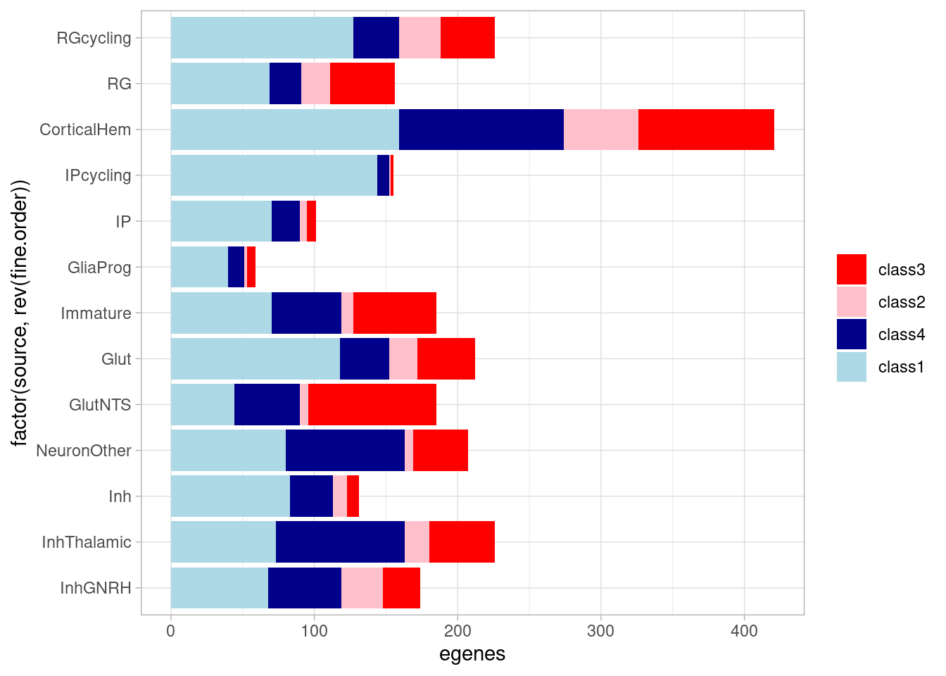

Past versions of unnamed-chunk-22-1.png

Version	Author	Date
f357871	Ben Umans	2025-02-24
f0eaf05	Ben Umans	2024-09-05

Our hypothesis is that the the dynamic effects that emerge under treatment should be less represented in GTEx, compared to effects that are evident at baseline, as GTEx does not (explicitly) assess gene expression under different environmental perturbations (although post-mortem brain tissue may experience some amount of hypoxia and/or hyperoxia during sample collection). While not testing for sharing of regulatory sites or effects here, we can ask whether these dynamic eGenes are less likely to be present in GTEx compared to the dynamic eGenes present at baseline.

mash_by_condition_output %>% 
  filter(sig_anywhere) %>% 
  mutate(class=case_when(control10_lfsr < 0.1 & allsharing ~ "class1",
                         control10_lfsr < 0.1 &  !allsharing ~ "class2",
                         sig_anywhere & control10_lfsr > 0.1 & !allsharing ~ "class3",
                         sig_anywhere & allsharing ~ "class4")) %>%  #because of the order of assignment, this does not include "class1" egenes, ie those that are detectable under normoxia.  equivalent to `allsharing & control10_lfsr > 0.1 & (stim1pct_lfsr < 0.1 | stim21pct_lfsr < 0.1) ~ "class4"`
   group_by(source, class) %>% 
  summarise(egene_gtex = sum(gene %in% gtex_cortex_signif),
            egene_in_gtex_fraction = round((sum(gene %in% gtex_cortex_signif))/n(), 4)) %>% 
  ggplot(aes(x=factor(class, levels = c("class1", "class4", "class2", "class3")), y=egene_in_gtex_fraction)) + 
  geom_boxplot(outlier.shape = NA, aes(color=class), linewidth=0.4) + 
  geom_point(aes(group=source, color=source), position = position_jitter(width = 0.2, height = 0), size=0.5) + 
  xlab("eGene class (see note)") + 
  ylab("Fraction of eGenes in GTEx") + 
  theme_light() +  
  scale_color_manual(values=c(manual_palette_fine, class_colors)) + theme(legend.position="none") 

`summarise()` has grouped output by 'source'. You can override using the
`.groups` argument.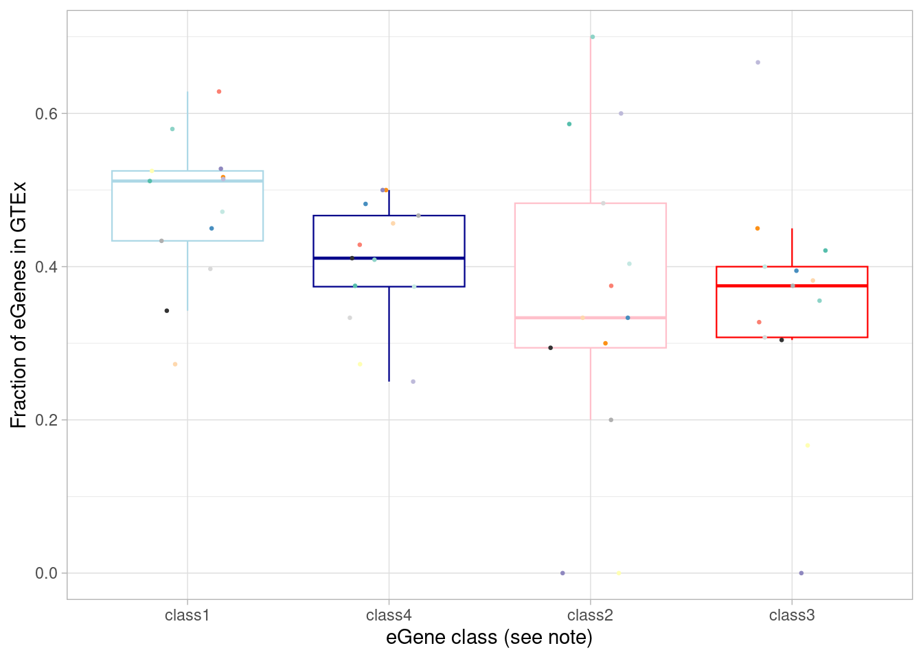

Past versions of unnamed-chunk-23-1.png

Version	Author	Date
f357871	Ben Umans	2025-02-24

To test the “class 3” (dynamic, not detected under normoxia) eGenes against the non-dynamic eGenes:

wilcox.test(mash_by_condition_output %>% 
  mutate(class=case_when(control10_lfsr < 0.1 & allsharing ~ "groupB",
                         control10_lfsr < 0.1 &  !allsharing ~ "groupB",
                         sig_anywhere & control10_lfsr > 0.1 & !allsharing ~ "groupA",
                         sig_anywhere & allsharing ~ "groupC", 
                         !sig_anywhere ~ "nonsig")) %>% 
    complete(source, class) %>% 
   group_by(source, class, .drop=FALSE) %>% 
    # filter(sig_anywhere) %>% 
  summarise(egene_gtex = sum(gene %in% (unlist(gtex_cortex_signif) %>% unique())),
            egene_in_gtex_fraction = (sum(gene %in% (unlist(gtex_cortex_signif) %>% unique())))/n()) %>% filter(class=="groupA") %>% pull(egene_in_gtex_fraction), 
  mash_by_condition_output %>% 
  filter(sig_anywhere) %>% 
  mutate(class=case_when(control10_lfsr < 0.1 & allsharing ~ "groupB",
                         control10_lfsr < 0.1 &  !allsharing ~ "groupB",
                         sig_anywhere & control10_lfsr > 0.1 & !allsharing ~ "groupA",
                         sig_anywhere & allsharing ~ "groupC")) %>% 
    complete(source, class) %>% 
   group_by(source, class, .drop=FALSE) %>% 
  summarise(egene_gtex = sum(gene %in% (unlist(gtex_cortex_signif) %>% unique())),
            egene_in_gtex_fraction = (sum(gene %in% (unlist(gtex_cortex_signif) %>% unique())))/n()) %>% filter(class %in% c("groupB")) %>% pull(egene_in_gtex_fraction), paired=TRUE,  alternative = "less")

`summarise()` has grouped output by 'source'. You can override using the
`.groups` argument.
`summarise()` has grouped output by 'source'. You can override using the
`.groups` argument.

    Wilcoxon signed rank exact test

data:  mash_by_condition_output %>% mutate(class = case_when(control10_lfsr < 0.1 & allsharing ~ "groupB", control10_lfsr < 0.1 & !allsharing ~ "groupB", sig_anywhere & control10_lfsr > 0.1 & !allsharing ~ "groupA", sig_anywhere & allsharing ~ "groupC", !sig_anywhere ~ "nonsig")) %>% complete(source, class) %>% group_by(source, class, .drop = FALSE) %>% summarise(egene_gtex = sum(gene %in% (unlist(gtex_cortex_signif) %>% unique())), egene_in_gtex_fraction = (sum(gene %in% (unlist(gtex_cortex_signif) %>%      unique())))/n()) %>% filter(class == "groupA") %>% pull(egene_in_gtex_fraction) and mash_by_condition_output %>% filter(sig_anywhere) %>% mutate(class = case_when(control10_lfsr < 0.1 & allsharing ~ "groupB", control10_lfsr < 0.1 & !allsharing ~ "groupB", sig_anywhere & control10_lfsr > 0.1 & !allsharing ~ "groupA", sig_anywhere & allsharing ~ "groupC")) %>% complete(source, class) %>% group_by(source, class, .drop = FALSE) %>% summarise(egene_gtex = sum(gene %in% (unlist(gtex_cortex_signif) %>% unique())), egene_in_gtex_fraction = (sum(gene %in% (unlist(gtex_cortex_signif) %>%      unique())))/n()) %>% filter(class %in% c("groupB")) %>% pull(egene_in_gtex_fraction)
V = 15, p-value = 0.01636
alternative hypothesis: true location shift is less than 0

The fraction of eGenes across cell types that would not be detected without treatment conditions is:

mash_by_condition_output %>% 
  filter(sig_anywhere) %>% 
 mutate(class=case_when(control10_lfsr < 0.1 & allsharing ~ "class1",
                         control10_lfsr < 0.1 &  !allsharing ~ "class2",
                         sig_anywhere & control10_lfsr > 0.1 & !allsharing ~ "class3",
                         allsharing & control10_lfsr > 0.1 & (stim1pct_lfsr < 0.1 | stim21pct_lfsr < 0.1) ~ "class4")) %>%  
  mutate(control_undetected=class %in% c("class3", "class4")) %>% 
  group_by(source) %>% 
  summarize(undetected_rate=sum(control_undetected)/n()) %>% 
  summarize(median(undetected_rate))

# A tibble: 1 × 1
  `median(undetected_rate)`
                      <dbl>
1                     0.429

The total number of eGenes detected here, in any condition or cell type, is:

mash_by_condition_output %>% 
  filter(sig_anywhere) %>%
  pull(gene) %>% 
  unique() %>%
  length()

[1] 1778

Many eGenes will have treatment-responsive effects in one cell type and treatment-shared effects in another cell type. The number of eGenes that have treatment-insensitive effects in at least one cell type is:

mash_by_condition_output %>% 
  filter(sig_anywhere) %>% 
  filter(allsharing) %>% 
  pull(gene) %>% 
  unique() %>%
  length()

[1] 1266

The number of eGenes that have treatment-sensitive effects in at least one cell type is:

mash_by_condition_output %>% 
  filter(sig_anywhere) %>% 
  filter(!allsharing) %>% 
  pull(gene) %>% 
  unique() %>%
  length()

[1] 658

Calculate the number of “dynamic” vs “standard” eQTLs per cell type, here defined by shared effect sizes. Note that because mash chooses a single eQTL/eGene in each cell type, within a cell type counting number of eGenes and eQTLs is equivalent.

mash_by_condition_output %>% 
  filter(sig_anywhere) %>% 
    group_by(source) %>% 
 mutate(class=case_when(allsharing ~ "allsharing",
                        hypoxia_normoxia_shared & sharing_contexts==1 ~ "hyperoxia_specific",
                        hyperoxia_normoxia_shared & sharing_contexts==1 ~ "hypoxia_specific",
                        hypoxia_hyperoxia_shared & sharing_contexts==1 ~ "normoxia_specific",
                        sharing_contexts==2 ~ "partial_shared", 
                        sharing_contexts==0 ~ "alldiff"
                        ),
        total=n(),
        standard=sum(allsharing)) %>%  
  mutate(dynamic=total-standard) %>% 
    ungroup() %>% 
    group_by(source, class) %>% 
    summarise(egene = n(), total=median(total), standard=median(standard), dynamic=median(dynamic)) %>% 
    mutate(fraction_total=egene/total, fraction_dynamic=egene/dynamic) %>% 
  ungroup() %>% 
    group_by(class) %>% 
  summarise(median(egene), median(total), median(dynamic), median(fraction_total), median(fraction_dynamic)) 

`summarise()` has grouped output by 'source'. You can override using the
`.groups` argument.

# A tibble: 6 × 6
  class `median(egene)` `median(total)` `median(dynamic)` median(fraction_tota…¹
  <chr>           <dbl>           <dbl>             <dbl>                  <dbl>
1 alld…              21             185              60                   0.0974
2 alls…             119             185              60                   0.717 
3 hype…               9             185              63                   0.0449
4 hypo…               5             185              61.5                 0.0362
5 norm…               6             185              63                   0.0380
6 part…               7             185              64                   0.0317
# ℹ abbreviated name: ¹​`median(fraction_total)`
# ℹ 1 more variable: `median(fraction_dynamic)` <dbl>

Here, anything that does not have a similar (ie, within 2-fold) effect size in all three oxygen conditions is called “dynamic”. Within this dynamic category we can define the following cases: * “treatment-shared” means different between normoxia and both hyperoxia and hypoxia, or, if you prefer, a normoxia-specific effect * “hypox_normox” means different in the hyperoxia condition from the other two * “hyperox_normox” means different in the hypoxia condition from the other two * “alldiff” means each oxygen condition has a different effect size from the other * “associatively_shared”, somewhat confusingly, means different between one pair of oxygen conditions but otherwise all shared. How can this happen? Consider a case where beta_normoxia=0.8, beta_hypoxia=0.4, and beta_hyperoxia=1.6. Here, both hypoxia and hyperoxia effects are shared with the normoxia condition (namely, differ by less than 2-fold), but differ from each other.

To plot these numbers:

class_colors3 <- c("allsharing"="blue", "partial_shared"="red", "normoxia_specific"="red", "hypoxia_specific"="red", "hyperoxia_specific"="red", "alldiff"="red")
mash_by_condition_output %>% 
  filter(sig_anywhere) %>% 
 mutate(class=case_when(allsharing ~ "allsharing",
                        hypoxia_normoxia_shared & sharing_contexts==1 ~ "hyperoxia_specific",
                        hyperoxia_normoxia_shared & sharing_contexts==1 ~ "hypoxia_specific",
                        hypoxia_hyperoxia_shared & sharing_contexts==1 ~ "normoxia_specific",
                        sharing_contexts==2 ~ "partial_shared", 
                        sharing_contexts==0 ~ "alldiff"
                        )) %>%   #because of the order of assignment, this does not include "class1" egenes, ie those that are detectable under normoxia.  equivalent to `allsharing & control10_lfsr > 0.1 & (stim1pct_lfsr < 0.1 | stim21pct_lfsr < 0.1) ~ "class4"`
   group_by(source, class) %>% 
  summarise(egene = n()) %>% 
  ggplot(aes(x=factor(class, levels=c("allsharing", "alldiff", "normoxia_specific", "hypoxia_specific", "hyperoxia_specific",  "partial_shared"), ordered = TRUE), y=egene)) + 
  geom_boxplot(outlier.shape = NA, aes(color=class)) + 
  geom_point(aes(group=source, color=source), position = position_jitter(width = 0.2, height = 0)) + 
  xlab("eGene class (see note)") + 
  ylab("Number of eGenes") + 
  theme_light() +  
  scale_color_manual(values=c(manual_palette_fine, class_colors3)) + theme(legend.position="none") 

`summarise()` has grouped output by 'source'. You can override using the
`.groups` argument.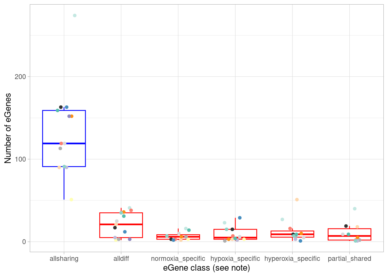

Past versions of unnamed-chunk-30-1.png

Version	Author	Date
f357871	Ben Umans	2025-02-24
f0eaf05	Ben Umans	2024-09-05

p1 <- mash_by_condition_output %>% 
  filter(sig_anywhere) %>% 
 mutate(class=case_when(allsharing ~ "allsharing",
                        hypoxia_normoxia_shared & sharing_contexts==1 ~ "hyperoxia_specific",
                        hyperoxia_normoxia_shared & sharing_contexts==1 ~ "hypoxia_specific",
                        hypoxia_hyperoxia_shared & sharing_contexts==1 ~ "normoxia_specific",
                        sharing_contexts==2 ~ "partial_shared", 
                        sharing_contexts==0 ~ "alldiff"
                        )) %>%   #because of the order of assignment, this does not include "class1" egenes, ie those that are detectable under normoxia.  equivalent to `allsharing & control10_lfsr > 0.1 & (stim1pct_lfsr < 0.1 | stim21pct_lfsr < 0.1) ~ "class4"`
   group_by(source, class) %>% 
  summarise(egene = n()) %>% 
  ggplot(aes(x=factor(class, levels=c("allsharing", "alldiff", "normoxia_specific", "hypoxia_specific", "hyperoxia_specific",  "partial_shared"), ordered = TRUE), y=egene)) + 
  geom_boxplot(outlier.shape = NA, aes(color=class), linewidth=0.4) + 
  geom_point(aes(group=source, color=source), position = position_jitter(width = 0.2, height = 0), size=0.3) + 
  xlab("eGene class (see note)") + 
  ylab("Number of eGenes") + 
  theme_light() +  
  scale_color_manual(values=c(manual_palette_fine, class_colors3)) + theme(legend.position="none") 

`summarise()` has grouped output by 'source'. You can override using the
`.groups` argument.

d1 <- mash_by_condition_output %>% 
  filter(sig_anywhere) %>% 
 mutate(class=case_when(allsharing ~ "allsharing",
                        hypoxia_normoxia_shared & sharing_contexts==1 ~ "hyperoxia_specific",
                        hyperoxia_normoxia_shared & sharing_contexts==1 ~ "hypoxia_specific",
                        hypoxia_hyperoxia_shared & sharing_contexts==1 ~ "normoxia_specific",
                        sharing_contexts==2 ~ "partial_shared", 
                        sharing_contexts==0 ~ "alldiff"
                        ),
        total=n(),
        standard=sum(allsharing)) %>%  
  mutate(dynamic=total-standard) %>% 
    group_by(class) %>% 
    summarise(egene = n(), total=median(total), standard=median(standard), dynamic=median(dynamic)) %>% 
    mutate(fraction_total=egene/total, fraction_dynamic=egene/dynamic) 


p1 + geom_point(aes(x=class, y=egene/7),  data = d1, shape=8, size=0.2) +
  scale_y_continuous(name = "eGenes per cell type", sec.axis = sec_axis(~ . *7, name="Total eQTLs"))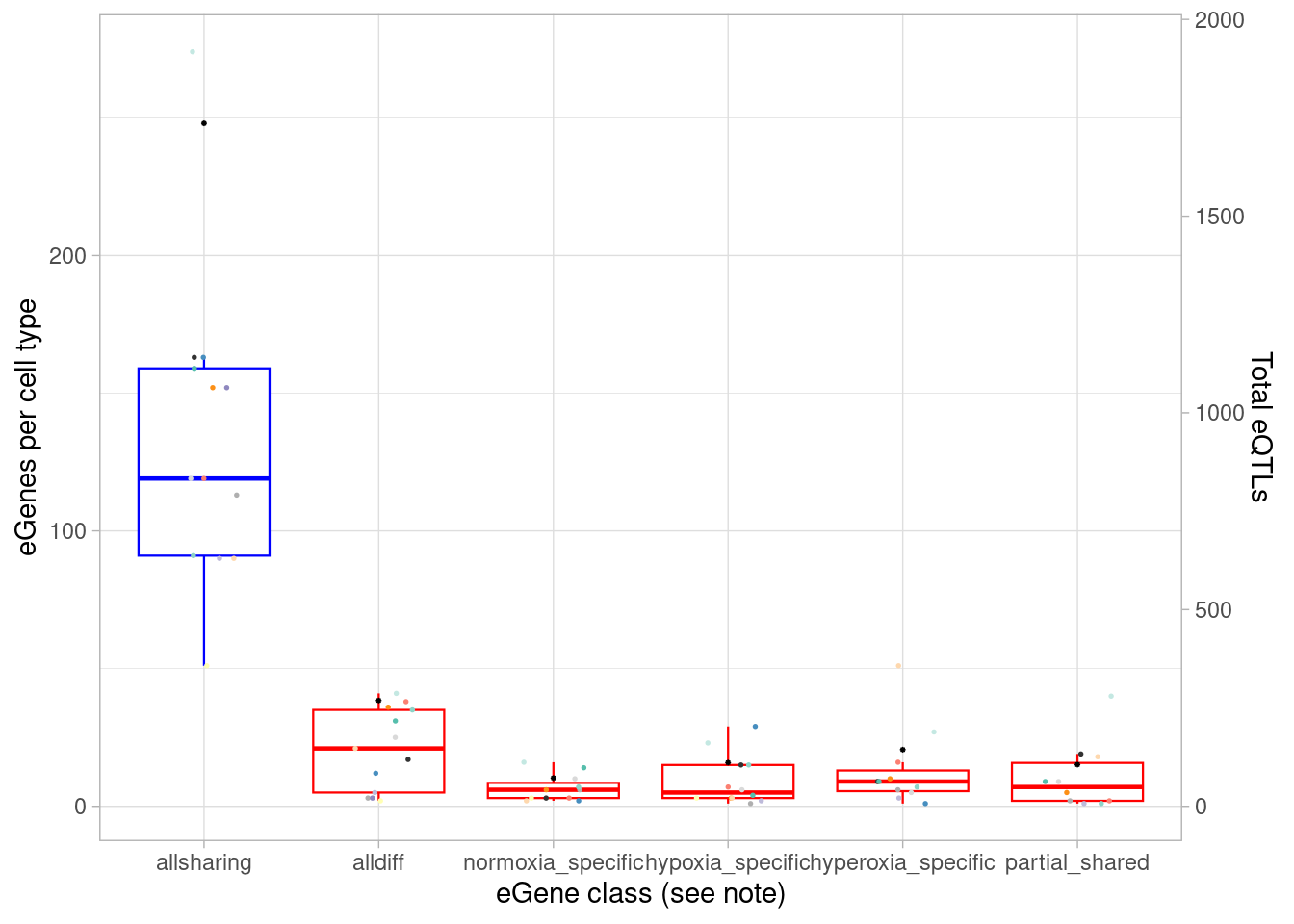 

Past versions of unnamed-chunk-31-1.png

Version	Author	Date
f357871	Ben Umans	2025-02-24

What fraction of each of these categories are in GTEx?

mash_by_condition_output %>% 
  filter(sig_anywhere) %>% 
 mutate(class=case_when(allsharing ~ "allsharing",
                        hypoxia_normoxia_shared & sharing_contexts==1 ~ "hyperoxia_specific",
                        hyperoxia_normoxia_shared & sharing_contexts==1 ~ "hypoxia_specific",
                        hypoxia_hyperoxia_shared & sharing_contexts==1 ~ "normoxia_specific",
                        sharing_contexts==2 ~ "partial_shared", 
                        sharing_contexts==0 ~ "alldiff"
                        )) %>%   #because of the order of assignment, this does not include "class1" egenes, ie those that are detectable under normoxia.  equivalent to `allsharing & control10_lfsr > 0.1 & (stim1pct_lfsr < 0.1 | stim21pct_lfsr < 0.1) ~ "class4"`
   group_by(source, class) %>% 
  summarise(egene_gtex = sum(gene %in% gtex_cortex_signif),
            egene_in_gtex_fraction = round((sum(gene %in% gtex_cortex_signif))/n(), 4)) %>% 
  ggplot(aes(x=factor(class, levels=c("allsharing", "partial_shared", "normoxia_specific", "hypoxia_specific", "hyperoxia_specific", "alldiff"), ordered = TRUE), y=egene_in_gtex_fraction)) + 
  geom_boxplot(outlier.shape = NA, aes(color=class), linewidth=0.4) + 
  geom_point(aes(group=source, color=source), position = position_jitter(width = 0.2, height = 0), size=0.5) + 
  xlab("eGene class (see note)") + 
  ylab("Fraction of eGenes in GTEx") + 
  theme_light() +  
  scale_color_manual(values=c(manual_palette_fine, class_colors)) + theme(legend.position="none") 

`summarise()` has grouped output by 'source'. You can override using the
`.groups` argument.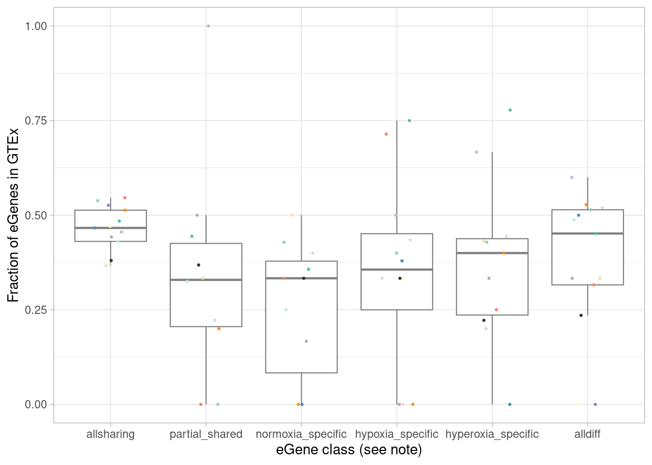

Past versions of unnamed-chunk-32-1.png

Version	Author	Date
f357871	Ben Umans	2025-02-24

We expect that the dynamic eGenes will be less represented in GTEx. To test this, I first designate the classes above as “standard” (all effects shared, or the strange case of all effects shared except for one comparison), or “dynamic”.

wilcox.test(mash_by_condition_output %>% 
 mutate(class=case_when(allsharing ~ "standard",
                        hypoxia_normoxia_shared & sharing_contexts==1 ~ "dynamic",
                        hyperoxia_normoxia_shared & sharing_contexts==1 ~ "dynamic",
                        hypoxia_hyperoxia_shared & sharing_contexts==1 ~ "dynamic",
                        sharing_contexts==2 ~ "standard", 
                        sharing_contexts==0 ~ "dynamic"
                        )) %>% 
   group_by(source, class, .drop = FALSE) %>% 
   filter(sig_anywhere) %>% 
   summarise(egene_gtex = sum(gene %in% (unlist(gtex_cortex_signif) %>% unique())),
            egene_in_gtex_fraction = (sum(gene %in% (unlist(gtex_cortex_signif) %>% unique())))/n()) %>%
   filter(class %in% c("dynamic")) %>% pull(egene_in_gtex_fraction), 
  mash_by_condition_output %>% 
  mutate(class=case_when(allsharing ~ "standard",
                        hypoxia_normoxia_shared & sharing_contexts==1 ~ "dynamic",
                        hyperoxia_normoxia_shared & sharing_contexts==1 ~ "dynamic",
                        hypoxia_hyperoxia_shared & sharing_contexts==1 ~ "dynamic",
                        sharing_contexts==2 ~ "standard", 
                        sharing_contexts==0 ~ "dynamic"
                        )) %>% 
   group_by(source, class, .drop = FALSE) %>% 
   filter(sig_anywhere) %>% 
  summarise(egene_gtex = sum(gene %in% (unlist(gtex_cortex_signif) %>% unique())),
            egene_in_gtex_fraction = (sum(gene %in% (unlist(gtex_cortex_signif) %>% unique())))/n()) %>%
   filter(class %in% c("standard")) %>% pull(egene_in_gtex_fraction), paired=TRUE, alternative = "less")

`summarise()` has grouped output by 'source'. You can override using the
`.groups` argument.
`summarise()` has grouped output by 'source'. You can override using the
`.groups` argument.

    Wilcoxon signed rank exact test

data:  mash_by_condition_output %>% mutate(class = case_when(allsharing ~ "standard", hypoxia_normoxia_shared & sharing_contexts == 1 ~ "dynamic", hyperoxia_normoxia_shared & sharing_contexts == 1 ~ "dynamic", hypoxia_hyperoxia_shared & sharing_contexts == 1 ~ "dynamic", sharing_contexts == 2 ~ "standard", sharing_contexts == 0 ~ "dynamic")) %>% group_by(source, class, .drop = FALSE) %>% filter(sig_anywhere) %>% summarise(egene_gtex = sum(gene %in% (unlist(gtex_cortex_signif) %>% unique())), egene_in_gtex_fraction = (sum(gene %in%      (unlist(gtex_cortex_signif) %>% unique())))/n()) %>% filter(class %in% c("dynamic")) %>% pull(egene_in_gtex_fraction) and mash_by_condition_output %>% mutate(class = case_when(allsharing ~ "standard", hypoxia_normoxia_shared & sharing_contexts == 1 ~ "dynamic", hyperoxia_normoxia_shared & sharing_contexts == 1 ~ "dynamic", hypoxia_hyperoxia_shared & sharing_contexts == 1 ~ "dynamic", sharing_contexts == 2 ~ "standard", sharing_contexts == 0 ~ "dynamic")) %>% group_by(source, class, .drop = FALSE) %>% filter(sig_anywhere) %>% summarise(egene_gtex = sum(gene %in% (unlist(gtex_cortex_signif) %>% unique())), egene_in_gtex_fraction = (sum(gene %in%      (unlist(gtex_cortex_signif) %>% unique())))/n()) %>% filter(class %in% c("standard")) %>% pull(egene_in_gtex_fraction)
V = 20, p-value = 0.04016
alternative hypothesis: true location shift is less than 0

Instead of counting per cell type, we can count total eQTLs:

mash_by_condition_output %>% 
  filter(sig_anywhere) %>% 
 mutate(class=case_when(allsharing ~ "allsharing",
                        hypoxia_normoxia_shared & sharing_contexts==1 ~ "hyperoxia_specific",
                        hyperoxia_normoxia_shared & sharing_contexts==1 ~ "hypoxia_specific",
                        hypoxia_hyperoxia_shared & sharing_contexts==1 ~ "normoxia_specific",
                        sharing_contexts==2 ~ "partial_shared", 
                        sharing_contexts==0 ~ "alldiff"
                        ),
        total=n(),
        standard=sum(allsharing)) %>%  
  mutate(dynamic=total-standard) %>% 
    group_by(class) %>% 
    summarise(egene = n(), total=median(total), standard=median(standard), dynamic=median(dynamic)) %>% 
    mutate(fraction_total=egene/total, fraction_dynamic=egene/dynamic) 

# A tibble: 6 × 7
  class             egene total standard dynamic fraction_total fraction_dynamic
  <chr>             <int> <dbl>    <dbl>   <dbl>          <dbl>            <dbl>
1 alldiff             269  2438     1736     702         0.110             0.383
2 allsharing         1736  2438     1736     702         0.712             2.47 
3 hyperoxia_specif…   144  2438     1736     702         0.0591            0.205
4 hypoxia_specific    111  2438     1736     702         0.0455            0.158
5 normoxia_specific    72  2438     1736     702         0.0295            0.103
6 partial_shared      106  2438     1736     702         0.0435            0.151

mash_by_condition_output %>% 
    filter(sig_anywhere) %>% group_by(gene) %>% summarise(eqtls=n()) %>%  summarise(mean(eqtls))

# A tibble: 1 × 1
  `mean(eqtls)`
          <dbl>
1          1.37

The number of eQTLs not detected in the control condition is:

mash_by_condition_output %>%
  filter(sig_anywhere) %>%
  filter(control10_lfsr>0.1) %>%
  nrow()

[1] 1088

And the number of response eQTLs not detected at baseline is:

mash_by_condition_output %>%
  filter(sig_anywhere) %>%
  filter(!allsharing) %>% 
  filter(control10_lfsr>0.1) %>%
  nrow()

[1] 497

To compare to primary tissue eQTLs more broadly, first I look across all GTEx tissues at at the recall rate of our organoid eGenes.

gtex_names <- list.files(path = "/project/gilad/umans/references/gtex/GTEx_Analysis_v8_eQTL", pattern="*.v8.egenes.txt.gz")

samplenums <- read_csv(file="/project2/gilad/umans/oxygen_eqtl/data/external/gtex_sample_numbers.csv", col_names = TRUE)

Rows: 50 Columns: 2
── Column specification ────────────────────────────────────────────────────────
Delimiter: ","
chr (1): Tissue
dbl (1): samples

ℹ Use `spec()` to retrieve the full column specification for this data.
ℹ Specify the column types or set `show_col_types = FALSE` to quiet this message.

egene_in_gtex <- c()
for (Y in gtex_names){
y <- read.table(file = paste0("/project/gilad/umans/references/gtex/GTEx_Analysis_v8_eQTL/", Y), header = TRUE, sep = "\t", stringsAsFactors = FALSE) %>% filter(qval<0.05)

egene_in_gtex[Y] <- mash_by_condition_output %>% 
  filter(sig_anywhere) %>% 
  select(gene) %>% distinct() %>% 
  summarize(sum(gene %in% y$gene_name)/n())
print(Y)
}

[1] "Adipose_Subcutaneous.v8.egenes.txt.gz"
[1] "Adipose_Visceral_Omentum.v8.egenes.txt.gz"
[1] "Adrenal_Gland.v8.egenes.txt.gz"
[1] "Artery_Aorta.v8.egenes.txt.gz"
[1] "Artery_Coronary.v8.egenes.txt.gz"
[1] "Artery_Tibial.v8.egenes.txt.gz"
[1] "Brain_Amygdala.v8.egenes.txt.gz"
[1] "Brain_Anterior_cingulate_cortex_BA24.v8.egenes.txt.gz"
[1] "Brain_Caudate_basal_ganglia.v8.egenes.txt.gz"
[1] "Brain_Cerebellar_Hemisphere.v8.egenes.txt.gz"
[1] "Brain_Cerebellum.v8.egenes.txt.gz"
[1] "Brain_Cortex.v8.egenes.txt.gz"
[1] "Brain_Frontal_Cortex_BA9.v8.egenes.txt.gz"
[1] "Brain_Hippocampus.v8.egenes.txt.gz"
[1] "Brain_Hypothalamus.v8.egenes.txt.gz"
[1] "Brain_Nucleus_accumbens_basal_ganglia.v8.egenes.txt.gz"
[1] "Brain_Putamen_basal_ganglia.v8.egenes.txt.gz"
[1] "Brain_Spinal_cord_cervical_c-1.v8.egenes.txt.gz"
[1] "Brain_Substantia_nigra.v8.egenes.txt.gz"
[1] "Breast_Mammary_Tissue.v8.egenes.txt.gz"
[1] "Cells_Cultured_fibroblasts.v8.egenes.txt.gz"
[1] "Cells_EBV-transformed_lymphocytes.v8.egenes.txt.gz"
[1] "Colon_Sigmoid.v8.egenes.txt.gz"
[1] "Colon_Transverse.v8.egenes.txt.gz"
[1] "Esophagus_Gastroesophageal_Junction.v8.egenes.txt.gz"
[1] "Esophagus_Mucosa.v8.egenes.txt.gz"
[1] "Esophagus_Muscularis.v8.egenes.txt.gz"
[1] "Heart_Atrial_Appendage.v8.egenes.txt.gz"
[1] "Heart_Left_Ventricle.v8.egenes.txt.gz"
[1] "Kidney_Cortex.v8.egenes.txt.gz"
[1] "Liver.v8.egenes.txt.gz"
[1] "Lung.v8.egenes.txt.gz"
[1] "Minor_Salivary_Gland.v8.egenes.txt.gz"
[1] "Muscle_Skeletal.v8.egenes.txt.gz"
[1] "Nerve_Tibial.v8.egenes.txt.gz"
[1] "Ovary.v8.egenes.txt.gz"
[1] "Pancreas.v8.egenes.txt.gz"
[1] "Pituitary.v8.egenes.txt.gz"
[1] "Prostate.v8.egenes.txt.gz"
[1] "Skin_Not_Sun_Exposed_Suprapubic.v8.egenes.txt.gz"
[1] "Skin_Sun_Exposed_Lower_leg.v8.egenes.txt.gz"
[1] "Small_Intestine_Terminal_Ileum.v8.egenes.txt.gz"
[1] "Spleen.v8.egenes.txt.gz"
[1] "Stomach.v8.egenes.txt.gz"
[1] "Testis.v8.egenes.txt.gz"
[1] "Thyroid.v8.egenes.txt.gz"
[1] "Uterus.v8.egenes.txt.gz"
[1] "Vagina.v8.egenes.txt.gz"
[1] "Whole_Blood.v8.egenes.txt.gz"

combined_egene_in_gtex <- egene_in_gtex %>%  bind_rows(.id = "tissue")

as_tibble(cbind(tissue = names(combined_egene_in_gtex), t(combined_egene_in_gtex))) %>% mutate(tissue=str_sub(tissue, end = -18)) %>% 
  mutate(V2=as.numeric(V2)) %>% left_join(samplenums, by=join_by("tissue"=="Tissue")) %>%
  ggplot(aes(x=reorder(tissue, V2), y=V2)) + 
  geom_point( size=0.5) + 
  scale_y_continuous(name = "Recall rate (black)", sec.axis = sec_axis(~ . *1000, name="GTEx sample size (red)")) +
  guides(x =  guide_axis(angle = 45)) +
  geom_point(aes(x=reorder(tissue, V2), y=samples/1000), color="red", size=0.5) + 
  theme_light() +coord_flip()

Warning: The `x` argument of `as_tibble.matrix()` must have unique column names if
`.name_repair` is omitted as of tibble 2.0.0.
ℹ Using compatibility `.name_repair`.
This warning is displayed once every 8 hours.
Call `lifecycle::last_lifecycle_warnings()` to see where this warning was
generated.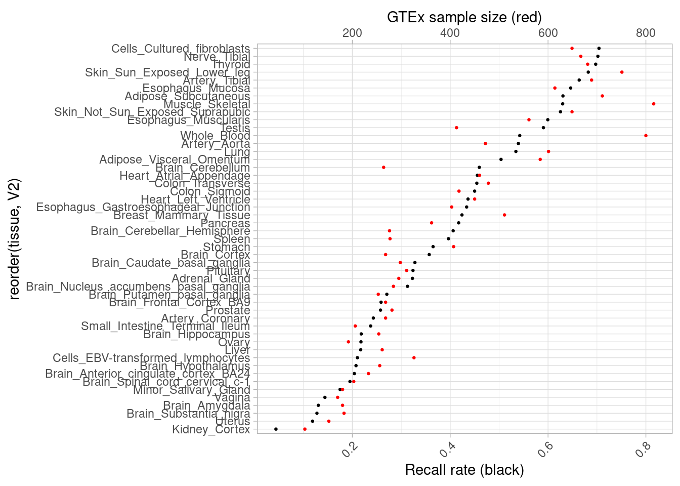

Past versions of unnamed-chunk-38-1.png

Version	Author	Date
f357871	Ben Umans	2025-02-24

Next, compare to the much larger Sieberts et al meta-analysis of CMC and AMP-AD cohorts.

cmc <- read_csv(file = "/project2/gilad/umans/oxygen_eqtl/data/external/Cortex_MetaAnalysis_ROSMAP_CMC_HBCC_Mayo_cis_eQTL_release.csv.gz", col_names = TRUE) %>% filter(FDR<0.05)

Rows: 100080618 Columns: 18
── Column specification ────────────────────────────────────────────────────────
Delimiter: ","
chr  (8): snpid, snpLocId, gene, geneSymbol, A1, A2, expressionIncreasingAll...
dbl (10): chromosome, snpLocation, statistic, pvalue, FDR, beta, A2freq, str...

ℹ Use `spec()` to retrieve the full column specification for this data.
ℹ Specify the column types or set `show_col_types = FALSE` to quiet this message.

mash_by_condition_output %>% 
  filter(sig_anywhere) %>% 
       mutate(class=case_when(allsharing ~ "standard",
                        hypoxia_normoxia_shared & sharing_contexts==1 ~ "hyperoxia_specific",
                        hyperoxia_normoxia_shared & sharing_contexts==1 ~ "hypoxia_specific",
                        hypoxia_hyperoxia_shared & sharing_contexts==1 ~ "normoxia_specific",
                        sharing_contexts==2 ~ "partial_shared", 
                        sharing_contexts==0 ~ "alldiff"
                        ) ) %>%  
   group_by(source, class) %>% 
      summarize(in_cmc = sum(gene %in% cmc$geneSymbol)/n()) %>% 
   ggplot(aes(y=source, x=class, fill=in_cmc)) + 
   geom_tile() + scale_fill_viridis(discrete=FALSE) + ggtitle("fraction of eGenes in CMC") + guides(x =  guide_axis(angle = 45)) + theme_light()

`summarise()` has grouped output by 'source'. You can override using the
`.groups` argument.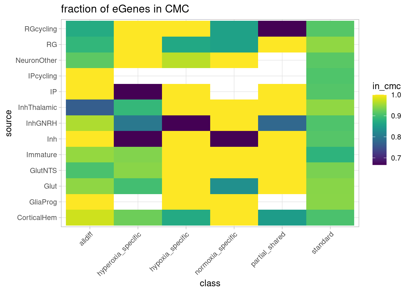

Past versions of unnamed-chunk-40-1.png

Version	Author	Date
f357871	Ben Umans	2025-02-24

Overall, this corresponds to

mash_by_condition_output %>% 
  filter(sig_anywhere) %>% 
  select(gene) %>% 
  distinct() %>% 
  summarize(in_cmc = sum(gene %in% cmc$geneSymbol)/n())

     in_cmc
1 0.9139483

of the eGenes identified in our study.

Finally, compare the estimated effect sizes of our eQTLs to the corresponding eQTLs in GTEx. Since mash only prioritizes a single SNP for each eGene in a given cell type (looking across all treaetment conditions), I’ll start by obtaining all additional SNPs with equal or better evidence (ie, smaller p-value than the mash-chosen variant) in the same condition and cell type in which we obtained an eQTL with lfsr<0.1.

controlset <- mash_by_condition_output %>% 
  filter(control10_lfsr<0.1) %>% 
  separate(gene_snp, into = c("genename", "snp"), sep = "_") %>% 
  # mutate(snp = str_sub(snp, end = -5)) %>% 
  select(snp, gene, source, control10_lfsr)
  
control_all_snps <- lapply(as.character(unique(controlset$source)), function(x) 
  controlset %>% filter(source==x) %>% #go cell type by cell type
    full_join(y=read.table(paste0("/project2/gilad/umans/oxygen_eqtl/data/MatrixEQTL/output/combined_fine_quality_filter20_032024/results_combined_control10_", x,"_nominal.txt.gz"), head=TRUE, stringsAsFactors=FALSE), by=join_by(gene, snp==snps)) %>% #join with original snp-gene pairs from which mash drew
    dplyr::filter(gene %in% (controlset %>% filter(source==x) %>% pull(gene))) %>% #filter to only those genes for which mash found a significant eqtl
    mutate(control10_lfsr=replace_na(control10_lfsr, replace = 0)) %>% #there will be a lfsr for only the mash lead variant.  set all others to 0
    group_by(gene) %>% 
    arrange(pvalue, control10_lfsr, .by_group = TRUE) %>% #first sort by ascending pvalue, then ascending lfsr. because we set the others to 0, this ensures we sort such that the mash lead variant comes last
    dplyr::slice(1:match(TRUE, !is.na(source))) %>% #take all of the snp-gene pairs up to the mash-chosen one
    select(snp, gene, pvalue, beta, lfsr=control10_lfsr) %>% 
    mutate(source=x)
  ) %>% bind_rows() %>% distinct() %>% 
  separate(snp, into = c("chrom", "position", "ref"), extra = "drop", sep = ":", convert = TRUE)

hypoxiaset <- mash_by_condition_output %>% 
  filter(stim1pct_lfsr < 0.1) %>% 
  separate(gene_snp, into = c("genename", "snp"), sep = "_") %>% 
  # mutate(snp = str_sub(snp, end = -5)) %>% 
  select(snp, gene, source, stim1pct_lfsr)

hypoxia_all_snps <- lapply(as.character(unique(hypoxiaset$source)), function(x) 
  hypoxiaset %>% filter(source==x) %>% full_join(y=read.table(paste0("/project2/gilad/umans/oxygen_eqtl/data/MatrixEQTL/output/combined_fine_quality_filter20_032024/results_combined_stim1pct_", x,"_nominal.txt.gz"), head=TRUE, stringsAsFactors=FALSE), by=join_by(gene, snp==snps)) %>% 
    dplyr::filter(gene %in% (hypoxiaset %>% filter(source==x) %>% pull(gene))) %>% 
    mutate(stim1pct_lfsr=replace_na(stim1pct_lfsr, replace = 0)) %>% 
    group_by(gene) %>% 
    arrange(pvalue, stim1pct_lfsr, .by_group = TRUE) %>% 
    dplyr::slice(1:match(TRUE, !is.na(source))) %>% 
    select(snp, gene, pvalue, beta, lfsr=stim1pct_lfsr) %>% 
    mutate(source=x)
  ) %>% bind_rows() %>% distinct() %>% 
  separate(snp, into = c("chrom", "position", "ref"), extra = "drop", sep = ":", convert = TRUE)

hyperoxiaset <- mash_by_condition_output %>% 
  filter(stim21pct_lfsr < 0.1) %>% 
  separate(gene_snp, into = c("genename", "snp"), sep = "_") %>% 
  # mutate(snp = str_sub(snp, end = -5)) %>% 
  select(snp, gene, source, stim21pct_lfsr)

hyperoxia_all_snps <- lapply(as.character(unique(hyperoxiaset$source)), function(x) 
  hyperoxiaset %>% filter(source==x) %>% full_join(y=read.table(paste0("/project2/gilad/umans/oxygen_eqtl/data/MatrixEQTL/output/combined_fine_quality_filter20_032024/results_combined_stim21pct_", x,"_nominal.txt.gz"), head=TRUE, stringsAsFactors=FALSE), by=join_by(gene, snp==snps)) %>% 
    dplyr::filter(gene %in% (hyperoxiaset %>% filter(source==x) %>% pull(gene))) %>% 
    mutate(stim21pct_lfsr=replace_na(stim21pct_lfsr, replace = 0)) %>% 
    group_by(gene) %>% 
    arrange(pvalue, stim21pct_lfsr, .by_group = TRUE) %>% 
    dplyr::slice(1:match(TRUE, !is.na(source))) %>% 
    select(snp, gene, pvalue, beta, lfsr=stim21pct_lfsr) %>% 
    mutate(source=x)
  ) %>% bind_rows() %>% distinct() %>% 
  separate(snp, into = c("chrom", "position", "ref"), extra = "drop", sep = ":", convert = TRUE)

combined_all_snpgenes <- bind_rows(control_all_snps, hypoxia_all_snps, hyperoxia_all_snps, .id = "treatment") %>% 
  ungroup() %>% 
  distinct()

rm(control_all_snps, hypoxia_all_snps, hyperoxia_all_snps)

Now, I go through all GTEx tissues, obtain significant eGenes and all corresponding eSNPs, then filter to the subset that correspond to our organoid results, and obtain a correlation.

gtex_names <- list.files(path = "/project/gilad/umans/references/gtex/GTEx_Analysis_v8_eQTL", pattern="*.v8.egenes.txt.gz")

gtex_beta_correlation_all <- list()
gtex_beta_ngenes_all <- numeric()
gtex_beta_correlation_all_combined <- numeric()

for (Y in gtex_names){
signif <- read.table(file = paste0("/project/gilad/umans/references/gtex/GTEx_Analysis_v8_eQTL/", Y), header = TRUE, sep = "\t", stringsAsFactors = FALSE) %>% filter(qval<0.05)

pairs <- read.table(file = paste0("/project/gilad/umans/references/gtex/GTEx_Analysis_v8_eQTL/", str_sub(Y, end=-14), "signif_variant_gene_pairs.txt.gz"), header = TRUE, sep = "\t", stringsAsFactors = FALSE)

joined <- pairs %>% 
  select(variant_id, gene_id, slope, pval_nominal) %>% 
  left_join(x=., y=signif %>% select(gene_id, gene_name), by=join_by( gene_id==gene_id), relationship="many-to-one") %>% 
  mutate(variant_id=str_sub(variant_id, start=4)) %>% 
  filter(str_detect(variant_id, "X_", negate = TRUE)) %>% #drop the X chromosome
  separate(variant_id, into = c("chrom", "position", "ref"), extra = "drop", sep="_", convert = TRUE) 

gtex_beta_correlation_all[[Y]] <- inner_join(combined_all_snpgenes, joined, by=join_by(gene==gene_name, chrom==chrom, position==position), relationship="many-to-many") %>% 
  group_by(source, treatment, .drop=FALSE) %>% 
  summarize(correlation=cor(beta, slope))
 
gtex_beta_ngenes_all[Y] <- inner_join(combined_all_snpgenes, joined, by=join_by(gene==gene_name, chrom==chrom, position==position), relationship="many-to-many") %>% 
  group_by(source, treatment, .drop=FALSE) %>% 
  summarize(n()) 

gtex_beta_correlation_all_combined[Y] <- inner_join(combined_all_snpgenes, joined, by=join_by(gene==gene_name, chrom==chrom, position==position), relationship="many-to-many") %>% 
  select(!source) %>% select(!lfsr) %>% 
  distinct() %>% 
  summarize(correlation=cor(beta, slope))

print(Y)
rm(signif, pairs, joined)
}

`summarise()` has grouped output by 'source'. You can override using the
`.groups` argument.
`summarise()` has grouped output by 'source'. You can override using the
`.groups` argument.

Warning in gtex_beta_ngenes_all[Y] <- inner_join(combined_all_snpgenes, :
number of items to replace is not a multiple of replacement length

[1] "Adipose_Subcutaneous.v8.egenes.txt.gz"

`summarise()` has grouped output by 'source'. You can override using the
`.groups` argument.
`summarise()` has grouped output by 'source'. You can override using the
`.groups` argument.

Warning in gtex_beta_ngenes_all[Y] <- inner_join(combined_all_snpgenes, :
number of items to replace is not a multiple of replacement length

[1] "Adipose_Visceral_Omentum.v8.egenes.txt.gz"

`summarise()` has grouped output by 'source'. You can override using the
`.groups` argument.
`summarise()` has grouped output by 'source'. You can override using the
`.groups` argument.

Warning in gtex_beta_ngenes_all[Y] <- inner_join(combined_all_snpgenes, :
number of items to replace is not a multiple of replacement length

[1] "Adrenal_Gland.v8.egenes.txt.gz"

`summarise()` has grouped output by 'source'. You can override using the
`.groups` argument.
`summarise()` has grouped output by 'source'. You can override using the
`.groups` argument.

Warning in gtex_beta_ngenes_all[Y] <- inner_join(combined_all_snpgenes, :
number of items to replace is not a multiple of replacement length

[1] "Artery_Aorta.v8.egenes.txt.gz"

`summarise()` has grouped output by 'source'. You can override using the
`.groups` argument.
`summarise()` has grouped output by 'source'. You can override using the
`.groups` argument.

Warning in gtex_beta_ngenes_all[Y] <- inner_join(combined_all_snpgenes, :
number of items to replace is not a multiple of replacement length

[1] "Artery_Coronary.v8.egenes.txt.gz"

`summarise()` has grouped output by 'source'. You can override using the
`.groups` argument.
`summarise()` has grouped output by 'source'. You can override using the
`.groups` argument.

Warning in gtex_beta_ngenes_all[Y] <- inner_join(combined_all_snpgenes, :
number of items to replace is not a multiple of replacement length

[1] "Artery_Tibial.v8.egenes.txt.gz"

`summarise()` has grouped output by 'source'. You can override using the
`.groups` argument.
`summarise()` has grouped output by 'source'. You can override using the
`.groups` argument.

Warning in gtex_beta_ngenes_all[Y] <- inner_join(combined_all_snpgenes, :
number of items to replace is not a multiple of replacement length

[1] "Brain_Amygdala.v8.egenes.txt.gz"

`summarise()` has grouped output by 'source'. You can override using the
`.groups` argument.
`summarise()` has grouped output by 'source'. You can override using the
`.groups` argument.

Warning in gtex_beta_ngenes_all[Y] <- inner_join(combined_all_snpgenes, :
number of items to replace is not a multiple of replacement length

[1] "Brain_Anterior_cingulate_cortex_BA24.v8.egenes.txt.gz"

`summarise()` has grouped output by 'source'. You can override using the
`.groups` argument.
`summarise()` has grouped output by 'source'. You can override using the
`.groups` argument.

Warning in gtex_beta_ngenes_all[Y] <- inner_join(combined_all_snpgenes, :
number of items to replace is not a multiple of replacement length

[1] "Brain_Caudate_basal_ganglia.v8.egenes.txt.gz"

`summarise()` has grouped output by 'source'. You can override using the
`.groups` argument.
`summarise()` has grouped output by 'source'. You can override using the
`.groups` argument.

Warning in gtex_beta_ngenes_all[Y] <- inner_join(combined_all_snpgenes, :
number of items to replace is not a multiple of replacement length

[1] "Brain_Cerebellar_Hemisphere.v8.egenes.txt.gz"

`summarise()` has grouped output by 'source'. You can override using the
`.groups` argument.
`summarise()` has grouped output by 'source'. You can override using the
`.groups` argument.

Warning in gtex_beta_ngenes_all[Y] <- inner_join(combined_all_snpgenes, :
number of items to replace is not a multiple of replacement length

[1] "Brain_Cerebellum.v8.egenes.txt.gz"

`summarise()` has grouped output by 'source'. You can override using the
`.groups` argument.
`summarise()` has grouped output by 'source'. You can override using the
`.groups` argument.

Warning in gtex_beta_ngenes_all[Y] <- inner_join(combined_all_snpgenes, :
number of items to replace is not a multiple of replacement length

[1] "Brain_Cortex.v8.egenes.txt.gz"

`summarise()` has grouped output by 'source'. You can override using the
`.groups` argument.
`summarise()` has grouped output by 'source'. You can override using the
`.groups` argument.

Warning in gtex_beta_ngenes_all[Y] <- inner_join(combined_all_snpgenes, :
number of items to replace is not a multiple of replacement length

[1] "Brain_Frontal_Cortex_BA9.v8.egenes.txt.gz"

`summarise()` has grouped output by 'source'. You can override using the
`.groups` argument.
`summarise()` has grouped output by 'source'. You can override using the
`.groups` argument.

Warning in gtex_beta_ngenes_all[Y] <- inner_join(combined_all_snpgenes, :
number of items to replace is not a multiple of replacement length

[1] "Brain_Hippocampus.v8.egenes.txt.gz"

`summarise()` has grouped output by 'source'. You can override using the
`.groups` argument.
`summarise()` has grouped output by 'source'. You can override using the
`.groups` argument.

Warning in gtex_beta_ngenes_all[Y] <- inner_join(combined_all_snpgenes, :
number of items to replace is not a multiple of replacement length

[1] "Brain_Hypothalamus.v8.egenes.txt.gz"

`summarise()` has grouped output by 'source'. You can override using the
`.groups` argument.
`summarise()` has grouped output by 'source'. You can override using the
`.groups` argument.

Warning in gtex_beta_ngenes_all[Y] <- inner_join(combined_all_snpgenes, :
number of items to replace is not a multiple of replacement length

[1] "Brain_Nucleus_accumbens_basal_ganglia.v8.egenes.txt.gz"

`summarise()` has grouped output by 'source'. You can override using the
`.groups` argument.
`summarise()` has grouped output by 'source'. You can override using the
`.groups` argument.

Warning in gtex_beta_ngenes_all[Y] <- inner_join(combined_all_snpgenes, :
number of items to replace is not a multiple of replacement length

[1] "Brain_Putamen_basal_ganglia.v8.egenes.txt.gz"

`summarise()` has grouped output by 'source'. You can override using the
`.groups` argument.
`summarise()` has grouped output by 'source'. You can override using the
`.groups` argument.

Warning in gtex_beta_ngenes_all[Y] <- inner_join(combined_all_snpgenes, :
number of items to replace is not a multiple of replacement length

[1] "Brain_Spinal_cord_cervical_c-1.v8.egenes.txt.gz"

Warning: There were 2 warnings in `summarize()`.
The first warning was:
ℹ In argument: `correlation = cor(beta, slope)`.
ℹ In group 26: `source = "InhGNRH"`, `treatment = "2"`.
Caused by warning in `cor()`:
! the standard deviation is zero
ℹ Run `dplyr::last_dplyr_warnings()` to see the 1 remaining warning.

`summarise()` has grouped output by 'source'. You can override using the
`.groups` argument.
`summarise()` has grouped output by 'source'. You can override using the
`.groups` argument.

Warning in gtex_beta_ngenes_all[Y] <- inner_join(combined_all_snpgenes, :
number of items to replace is not a multiple of replacement length

[1] "Brain_Substantia_nigra.v8.egenes.txt.gz"

`summarise()` has grouped output by 'source'. You can override using the
`.groups` argument.
`summarise()` has grouped output by 'source'. You can override using the
`.groups` argument.

Warning in gtex_beta_ngenes_all[Y] <- inner_join(combined_all_snpgenes, :
number of items to replace is not a multiple of replacement length

[1] "Breast_Mammary_Tissue.v8.egenes.txt.gz"

`summarise()` has grouped output by 'source'. You can override using the
`.groups` argument.
`summarise()` has grouped output by 'source'. You can override using the
`.groups` argument.

Warning in gtex_beta_ngenes_all[Y] <- inner_join(combined_all_snpgenes, :
number of items to replace is not a multiple of replacement length

[1] "Cells_Cultured_fibroblasts.v8.egenes.txt.gz"

`summarise()` has grouped output by 'source'. You can override using the
`.groups` argument.
`summarise()` has grouped output by 'source'. You can override using the
`.groups` argument.

Warning in gtex_beta_ngenes_all[Y] <- inner_join(combined_all_snpgenes, :
number of items to replace is not a multiple of replacement length

[1] "Cells_EBV-transformed_lymphocytes.v8.egenes.txt.gz"

`summarise()` has grouped output by 'source'. You can override using the
`.groups` argument.
`summarise()` has grouped output by 'source'. You can override using the
`.groups` argument.

Warning in gtex_beta_ngenes_all[Y] <- inner_join(combined_all_snpgenes, :
number of items to replace is not a multiple of replacement length

[1] "Colon_Sigmoid.v8.egenes.txt.gz"

`summarise()` has grouped output by 'source'. You can override using the
`.groups` argument.
`summarise()` has grouped output by 'source'. You can override using the
`.groups` argument.

Warning in gtex_beta_ngenes_all[Y] <- inner_join(combined_all_snpgenes, :
number of items to replace is not a multiple of replacement length

[1] "Colon_Transverse.v8.egenes.txt.gz"

`summarise()` has grouped output by 'source'. You can override using the
`.groups` argument.
`summarise()` has grouped output by 'source'. You can override using the
`.groups` argument.

Warning in gtex_beta_ngenes_all[Y] <- inner_join(combined_all_snpgenes, :
number of items to replace is not a multiple of replacement length

[1] "Esophagus_Gastroesophageal_Junction.v8.egenes.txt.gz"

`summarise()` has grouped output by 'source'. You can override using the
`.groups` argument.
`summarise()` has grouped output by 'source'. You can override using the
`.groups` argument.

Warning in gtex_beta_ngenes_all[Y] <- inner_join(combined_all_snpgenes, :
number of items to replace is not a multiple of replacement length

[1] "Esophagus_Mucosa.v8.egenes.txt.gz"

`summarise()` has grouped output by 'source'. You can override using the
`.groups` argument.
`summarise()` has grouped output by 'source'. You can override using the
`.groups` argument.

Warning in gtex_beta_ngenes_all[Y] <- inner_join(combined_all_snpgenes, :
number of items to replace is not a multiple of replacement length

[1] "Esophagus_Muscularis.v8.egenes.txt.gz"

`summarise()` has grouped output by 'source'. You can override using the
`.groups` argument.
`summarise()` has grouped output by 'source'. You can override using the
`.groups` argument.

Warning in gtex_beta_ngenes_all[Y] <- inner_join(combined_all_snpgenes, :
number of items to replace is not a multiple of replacement length

[1] "Heart_Atrial_Appendage.v8.egenes.txt.gz"

`summarise()` has grouped output by 'source'. You can override using the
`.groups` argument.
`summarise()` has grouped output by 'source'. You can override using the
`.groups` argument.

Warning in gtex_beta_ngenes_all[Y] <- inner_join(combined_all_snpgenes, :
number of items to replace is not a multiple of replacement length

[1] "Heart_Left_Ventricle.v8.egenes.txt.gz"

Warning: There were 3 warnings in `summarize()`.
The first warning was:
ℹ In argument: `correlation = cor(beta, slope)`.
ℹ In group 11: `source = "GlutNTS"`, `treatment = "3"`.
Caused by warning in `cor()`:
! the standard deviation is zero
ℹ Run `dplyr::last_dplyr_warnings()` to see the 2 remaining warnings.

`summarise()` has grouped output by 'source'. You can override using the
`.groups` argument.
`summarise()` has grouped output by 'source'. You can override using the
`.groups` argument.

Warning in gtex_beta_ngenes_all[Y] <- inner_join(combined_all_snpgenes, :
number of items to replace is not a multiple of replacement length

[1] "Kidney_Cortex.v8.egenes.txt.gz"

`summarise()` has grouped output by 'source'. You can override using the
`.groups` argument.
`summarise()` has grouped output by 'source'. You can override using the
`.groups` argument.

Warning in gtex_beta_ngenes_all[Y] <- inner_join(combined_all_snpgenes, :
number of items to replace is not a multiple of replacement length

[1] "Liver.v8.egenes.txt.gz"

`summarise()` has grouped output by 'source'. You can override using the
`.groups` argument.
`summarise()` has grouped output by 'source'. You can override using the
`.groups` argument.

Warning in gtex_beta_ngenes_all[Y] <- inner_join(combined_all_snpgenes, :
number of items to replace is not a multiple of replacement length

[1] "Lung.v8.egenes.txt.gz"

Warning: There was 1 warning in `summarize()`.
ℹ In argument: `correlation = cor(beta, slope)`.
ℹ In group 25: `source = "InhGNRH"`, `treatment = "1"`.
Caused by warning in `cor()`:
! the standard deviation is zero

`summarise()` has grouped output by 'source'. You can override using the
`.groups` argument.
`summarise()` has grouped output by 'source'. You can override using the
`.groups` argument.

Warning in gtex_beta_ngenes_all[Y] <- inner_join(combined_all_snpgenes, :
number of items to replace is not a multiple of replacement length

[1] "Minor_Salivary_Gland.v8.egenes.txt.gz"

`summarise()` has grouped output by 'source'. You can override using the
`.groups` argument.
`summarise()` has grouped output by 'source'. You can override using the
`.groups` argument.

Warning in gtex_beta_ngenes_all[Y] <- inner_join(combined_all_snpgenes, :
number of items to replace is not a multiple of replacement length

[1] "Muscle_Skeletal.v8.egenes.txt.gz"

`summarise()` has grouped output by 'source'. You can override using the
`.groups` argument.
`summarise()` has grouped output by 'source'. You can override using the
`.groups` argument.

Warning in gtex_beta_ngenes_all[Y] <- inner_join(combined_all_snpgenes, :
number of items to replace is not a multiple of replacement length

[1] "Nerve_Tibial.v8.egenes.txt.gz"

`summarise()` has grouped output by 'source'. You can override using the
`.groups` argument.
`summarise()` has grouped output by 'source'. You can override using the
`.groups` argument.

Warning in gtex_beta_ngenes_all[Y] <- inner_join(combined_all_snpgenes, :
number of items to replace is not a multiple of replacement length

[1] "Ovary.v8.egenes.txt.gz"

`summarise()` has grouped output by 'source'. You can override using the
`.groups` argument.
`summarise()` has grouped output by 'source'. You can override using the
`.groups` argument.

Warning in gtex_beta_ngenes_all[Y] <- inner_join(combined_all_snpgenes, :
number of items to replace is not a multiple of replacement length

[1] "Pancreas.v8.egenes.txt.gz"

`summarise()` has grouped output by 'source'. You can override using the
`.groups` argument.
`summarise()` has grouped output by 'source'. You can override using the
`.groups` argument.

Warning in gtex_beta_ngenes_all[Y] <- inner_join(combined_all_snpgenes, :
number of items to replace is not a multiple of replacement length

[1] "Pituitary.v8.egenes.txt.gz"

`summarise()` has grouped output by 'source'. You can override using the
`.groups` argument.
`summarise()` has grouped output by 'source'. You can override using the
`.groups` argument.

Warning in gtex_beta_ngenes_all[Y] <- inner_join(combined_all_snpgenes, :
number of items to replace is not a multiple of replacement length

[1] "Prostate.v8.egenes.txt.gz"

`summarise()` has grouped output by 'source'. You can override using the
`.groups` argument.
`summarise()` has grouped output by 'source'. You can override using the
`.groups` argument.

Warning in gtex_beta_ngenes_all[Y] <- inner_join(combined_all_snpgenes, :
number of items to replace is not a multiple of replacement length

[1] "Skin_Not_Sun_Exposed_Suprapubic.v8.egenes.txt.gz"

`summarise()` has grouped output by 'source'. You can override using the
`.groups` argument.
`summarise()` has grouped output by 'source'. You can override using the
`.groups` argument.

Warning in gtex_beta_ngenes_all[Y] <- inner_join(combined_all_snpgenes, :
number of items to replace is not a multiple of replacement length

[1] "Skin_Sun_Exposed_Lower_leg.v8.egenes.txt.gz"

`summarise()` has grouped output by 'source'. You can override using the
`.groups` argument.
`summarise()` has grouped output by 'source'. You can override using the
`.groups` argument.

Warning in gtex_beta_ngenes_all[Y] <- inner_join(combined_all_snpgenes, :
number of items to replace is not a multiple of replacement length

[1] "Small_Intestine_Terminal_Ileum.v8.egenes.txt.gz"

`summarise()` has grouped output by 'source'. You can override using the
`.groups` argument.
`summarise()` has grouped output by 'source'. You can override using the
`.groups` argument.

Warning in gtex_beta_ngenes_all[Y] <- inner_join(combined_all_snpgenes, :
number of items to replace is not a multiple of replacement length

[1] "Spleen.v8.egenes.txt.gz"

`summarise()` has grouped output by 'source'. You can override using the
`.groups` argument.
`summarise()` has grouped output by 'source'. You can override using the
`.groups` argument.

Warning in gtex_beta_ngenes_all[Y] <- inner_join(combined_all_snpgenes, :
number of items to replace is not a multiple of replacement length

[1] "Stomach.v8.egenes.txt.gz"

`summarise()` has grouped output by 'source'. You can override using the
`.groups` argument.
`summarise()` has grouped output by 'source'. You can override using the
`.groups` argument.

Warning in gtex_beta_ngenes_all[Y] <- inner_join(combined_all_snpgenes, :
number of items to replace is not a multiple of replacement length

[1] "Testis.v8.egenes.txt.gz"

`summarise()` has grouped output by 'source'. You can override using the
`.groups` argument.
`summarise()` has grouped output by 'source'. You can override using the
`.groups` argument.

Warning in gtex_beta_ngenes_all[Y] <- inner_join(combined_all_snpgenes, :
number of items to replace is not a multiple of replacement length

[1] "Thyroid.v8.egenes.txt.gz"

Warning: There was 1 warning in `summarize()`.
ℹ In argument: `correlation = cor(beta, slope)`.
ℹ In group 25: `source = "InhGNRH"`, `treatment = "1"`.
Caused by warning in `cor()`:
! the standard deviation is zero

`summarise()` has grouped output by 'source'. You can override using the
`.groups` argument.
`summarise()` has grouped output by 'source'. You can override using the
`.groups` argument.

Warning in gtex_beta_ngenes_all[Y] <- inner_join(combined_all_snpgenes, :
number of items to replace is not a multiple of replacement length

[1] "Uterus.v8.egenes.txt.gz"

`summarise()` has grouped output by 'source'. You can override using the
`.groups` argument.
`summarise()` has grouped output by 'source'. You can override using the
`.groups` argument.

Warning in gtex_beta_ngenes_all[Y] <- inner_join(combined_all_snpgenes, :
number of items to replace is not a multiple of replacement length

[1] "Vagina.v8.egenes.txt.gz"

`summarise()` has grouped output by 'source'. You can override using the
`.groups` argument.
`summarise()` has grouped output by 'source'. You can override using the
`.groups` argument.

Warning in gtex_beta_ngenes_all[Y] <- inner_join(combined_all_snpgenes, :
number of items to replace is not a multiple of replacement length

[1] "Whole_Blood.v8.egenes.txt.gz"

gtex_beta_correlation_all %>%  bind_rows(.id = "tissue") %>% mutate(tissue=str_sub(tissue, end = -18)) %>% 
  filter(treatment==1) %>% 
   ggplot(aes(x=source, y=tissue, fill=correlation)) + 
   geom_tile() + scale_fill_viridis(discrete=FALSE, limits = c(-1, 1)) + ggtitle("Significant in control") + guides(x =  guide_axis(angle = 45))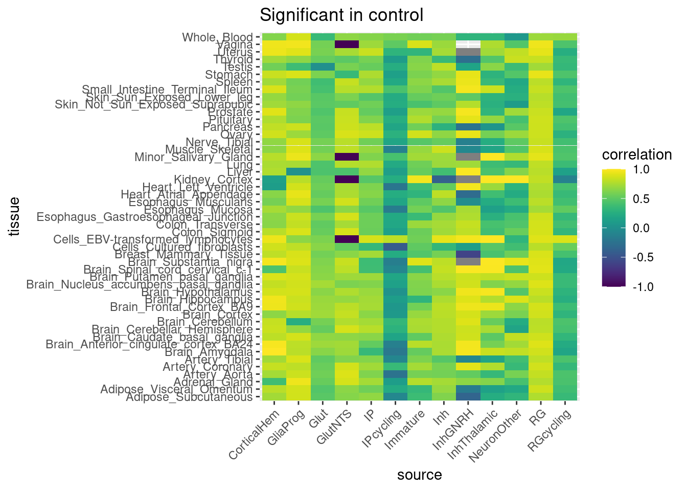

Past versions of unnamed-chunk-43-1.png

Version	Author	Date
f357871	Ben Umans	2025-02-24
f0eaf05	Ben Umans	2024-09-05

gtex_beta_correlation_all %>%  bind_rows(.id = "tissue") %>% mutate(tissue=str_sub(tissue, end = -18)) %>% 
  filter(treatment==2) %>% 
   ggplot(aes(x=source, y=tissue, fill=correlation)) + 
   geom_tile() + scale_fill_viridis(discrete=FALSE, limits = c(-1, 1)) + ggtitle("Significant in hypoxia") + guides(x =  guide_axis(angle = 45))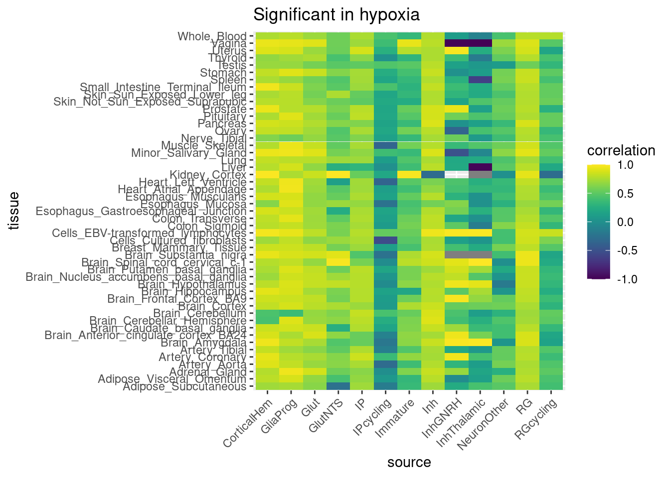

gtex_beta_correlation_all %>%  bind_rows(.id = "tissue") %>% mutate(tissue=str_sub(tissue, end = -18)) %>% 
  filter(treatment==3) %>% 
   ggplot(aes(x=source, y=tissue, fill=correlation)) + 
   geom_tile() + scale_fill_viridis(discrete=FALSE, limits = c(-1, 1)) + ggtitle("Significant in hyperoxia") + guides(x =  guide_axis(angle = 45))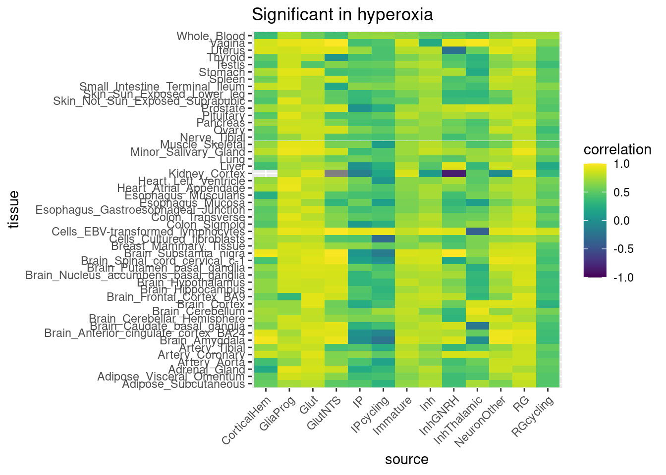

The actual numbers here are:

gtex_beta_correlation_all_combined 

$Adipose_Subcutaneous.v8.egenes.txt.gz
[1] 0.3990559

$Adipose_Visceral_Omentum.v8.egenes.txt.gz
[1] 0.5450481

$Adrenal_Gland.v8.egenes.txt.gz
[1] 0.5746033

$Artery_Aorta.v8.egenes.txt.gz
[1] 0.392625

$Artery_Coronary.v8.egenes.txt.gz
[1] 0.6257047

$Artery_Tibial.v8.egenes.txt.gz
[1] 0.4568482

$Brain_Amygdala.v8.egenes.txt.gz
[1] 0.5023542

$Brain_Anterior_cingulate_cortex_BA24.v8.egenes.txt.gz
[1] 0.5774967

$Brain_Caudate_basal_ganglia.v8.egenes.txt.gz
[1] 0.5683777

$Brain_Cerebellar_Hemisphere.v8.egenes.txt.gz
[1] 0.60424

$Brain_Cerebellum.v8.egenes.txt.gz
[1] 0.6105223

$Brain_Cortex.v8.egenes.txt.gz
[1] 0.5772053

$Brain_Frontal_Cortex_BA9.v8.egenes.txt.gz
[1] 0.6008969

$Brain_Hippocampus.v8.egenes.txt.gz
[1] 0.5486654

$Brain_Hypothalamus.v8.egenes.txt.gz
[1] 0.58624

$Brain_Nucleus_accumbens_basal_ganglia.v8.egenes.txt.gz
[1] 0.5921205

$Brain_Putamen_basal_ganglia.v8.egenes.txt.gz
[1] 0.5985901

$`Brain_Spinal_cord_cervical_c-1.v8.egenes.txt.gz`
[1] 0.5489082

$Brain_Substantia_nigra.v8.egenes.txt.gz
[1] 0.5810231

$Breast_Mammary_Tissue.v8.egenes.txt.gz
[1] 0.6063023

$Cells_Cultured_fibroblasts.v8.egenes.txt.gz
[1] 0.1949566

$`Cells_EBV-transformed_lymphocytes.v8.egenes.txt.gz`
[1] 0.8133432

$Colon_Sigmoid.v8.egenes.txt.gz
[1] 0.5612438

$Colon_Transverse.v8.egenes.txt.gz
[1] 0.5965302

$Esophagus_Gastroesophageal_Junction.v8.egenes.txt.gz
[1] 0.5449756

$Esophagus_Mucosa.v8.egenes.txt.gz
[1] 0.3540216

$Esophagus_Muscularis.v8.egenes.txt.gz
[1] 0.5316953

$Heart_Atrial_Appendage.v8.egenes.txt.gz
[1] 0.561822

$Heart_Left_Ventricle.v8.egenes.txt.gz
[1] 0.3360566

$Kidney_Cortex.v8.egenes.txt.gz
[1] 0.4139731

$Liver.v8.egenes.txt.gz
[1] 0.4708509

$Lung.v8.egenes.txt.gz
[1] 0.5531796

$Minor_Salivary_Gland.v8.egenes.txt.gz
[1] 0.6656595

$Muscle_Skeletal.v8.egenes.txt.gz
[1] 0.4703824

$Nerve_Tibial.v8.egenes.txt.gz
[1] 0.5247274

$Ovary.v8.egenes.txt.gz
[1] 0.5932552

$Pancreas.v8.egenes.txt.gz
[1] 0.5765865

$Pituitary.v8.egenes.txt.gz
[1] 0.6220919

$Prostate.v8.egenes.txt.gz
[1] 0.5550918

$Skin_Not_Sun_Exposed_Suprapubic.v8.egenes.txt.gz
[1] 0.5375844

$Skin_Sun_Exposed_Lower_leg.v8.egenes.txt.gz
[1] 0.5276979

$Small_Intestine_Terminal_Ileum.v8.egenes.txt.gz
[1] 0.6090839

$Spleen.v8.egenes.txt.gz
[1] 0.5484934

$Stomach.v8.egenes.txt.gz
[1] 0.613231

$Testis.v8.egenes.txt.gz
[1] 0.4697669

$Thyroid.v8.egenes.txt.gz
[1] 0.5051611

$Uterus.v8.egenes.txt.gz
[1] 0.6052053

$Vagina.v8.egenes.txt.gz
[1] 0.6569809

$Whole_Blood.v8.egenes.txt.gz
[1] 0.6217828

And these are based on a reasonable number of genes:

gtex_beta_ngenes_all 

$Adipose_Subcutaneous.v8.egenes.txt.gz
 [1] "CorticalHem" "CorticalHem" "CorticalHem" "GliaProg"    "GliaProg"   
 [6] "GliaProg"    "Glut"        "Glut"        "Glut"        "GlutNTS"    
[11] "GlutNTS"     "GlutNTS"     "IP"          "IP"          "IP"         
[16] "IPcycling"   "IPcycling"   "IPcycling"   "Immature"    "Immature"   
[21] "Immature"    "Inh"         "Inh"         "Inh"         "InhGNRH"    
[26] "InhGNRH"     "InhGNRH"     "InhThalamic" "InhThalamic" "InhThalamic"
[31] "NeuronOther" "NeuronOther" "NeuronOther" "RG"          "RG"         
[36] "RG"          "RGcycling"   "RGcycling"   "RGcycling"  

$Adipose_Visceral_Omentum.v8.egenes.txt.gz
 [1] "CorticalHem" "CorticalHem" "CorticalHem" "GliaProg"    "GliaProg"   
 [6] "GliaProg"    "Glut"        "Glut"        "Glut"        "GlutNTS"    
[11] "GlutNTS"     "GlutNTS"     "IP"          "IP"          "IP"         
[16] "IPcycling"   "IPcycling"   "IPcycling"   "Immature"    "Immature"   
[21] "Immature"    "Inh"         "Inh"         "Inh"         "InhGNRH"    
[26] "InhGNRH"     "InhGNRH"     "InhThalamic" "InhThalamic" "InhThalamic"
[31] "NeuronOther" "NeuronOther" "NeuronOther" "RG"          "RG"         
[36] "RG"          "RGcycling"   "RGcycling"   "RGcycling"  

$Adrenal_Gland.v8.egenes.txt.gz
 [1] "CorticalHem" "CorticalHem" "CorticalHem" "GliaProg"    "GliaProg"   
 [6] "GliaProg"    "Glut"        "Glut"        "Glut"        "GlutNTS"    
[11] "GlutNTS"     "GlutNTS"     "IP"          "IP"          "IP"         
[16] "IPcycling"   "IPcycling"   "IPcycling"   "Immature"    "Immature"   
[21] "Immature"    "Inh"         "Inh"         "Inh"         "InhGNRH"    
[26] "InhGNRH"     "InhGNRH"     "InhThalamic" "InhThalamic" "InhThalamic"
[31] "NeuronOther" "NeuronOther" "NeuronOther" "RG"          "RG"         
[36] "RG"          "RGcycling"   "RGcycling"   "RGcycling"  

$Artery_Aorta.v8.egenes.txt.gz
 [1] "CorticalHem" "CorticalHem" "CorticalHem" "GliaProg"    "GliaProg"   
 [6] "GliaProg"    "Glut"        "Glut"        "Glut"        "GlutNTS"    
[11] "GlutNTS"     "GlutNTS"     "IP"          "IP"          "IP"         
[16] "IPcycling"   "IPcycling"   "IPcycling"   "Immature"    "Immature"   
[21] "Immature"    "Inh"         "Inh"         "Inh"         "InhGNRH"    
[26] "InhGNRH"     "InhGNRH"     "InhThalamic" "InhThalamic" "InhThalamic"
[31] "NeuronOther" "NeuronOther" "NeuronOther" "RG"          "RG"         
[36] "RG"          "RGcycling"   "RGcycling"   "RGcycling"  

$Artery_Coronary.v8.egenes.txt.gz
 [1] "CorticalHem" "CorticalHem" "CorticalHem" "GliaProg"    "GliaProg"   
 [6] "GliaProg"    "Glut"        "Glut"        "Glut"        "GlutNTS"    
[11] "GlutNTS"     "GlutNTS"     "IP"          "IP"          "IP"         
[16] "IPcycling"   "IPcycling"   "IPcycling"   "Immature"    "Immature"   
[21] "Immature"    "Inh"         "Inh"         "Inh"         "InhGNRH"    
[26] "InhGNRH"     "InhGNRH"     "InhThalamic" "InhThalamic" "InhThalamic"
[31] "NeuronOther" "NeuronOther" "NeuronOther" "RG"          "RG"         
[36] "RG"          "RGcycling"   "RGcycling"   "RGcycling"  

$Artery_Tibial.v8.egenes.txt.gz
 [1] "CorticalHem" "CorticalHem" "CorticalHem" "GliaProg"    "GliaProg"   
 [6] "GliaProg"    "Glut"        "Glut"        "Glut"        "GlutNTS"    
[11] "GlutNTS"     "GlutNTS"     "IP"          "IP"          "IP"         
[16] "IPcycling"   "IPcycling"   "IPcycling"   "Immature"    "Immature"   
[21] "Immature"    "Inh"         "Inh"         "Inh"         "InhGNRH"    
[26] "InhGNRH"     "InhGNRH"     "InhThalamic" "InhThalamic" "InhThalamic"
[31] "NeuronOther" "NeuronOther" "NeuronOther" "RG"          "RG"         
[36] "RG"          "RGcycling"   "RGcycling"   "RGcycling"  

$Brain_Amygdala.v8.egenes.txt.gz
 [1] "CorticalHem" "CorticalHem" "CorticalHem" "GliaProg"    "GliaProg"   
 [6] "GliaProg"    "Glut"        "Glut"        "Glut"        "GlutNTS"    
[11] "GlutNTS"     "GlutNTS"     "IP"          "IP"          "IP"         
[16] "IPcycling"   "IPcycling"   "IPcycling"   "Immature"    "Immature"   
[21] "Immature"    "Inh"         "Inh"         "Inh"         "InhGNRH"    
[26] "InhGNRH"     "InhGNRH"     "InhThalamic" "InhThalamic" "InhThalamic"
[31] "NeuronOther" "NeuronOther" "NeuronOther" "RG"          "RG"         
[36] "RG"          "RGcycling"   "RGcycling"   "RGcycling"  

$Brain_Anterior_cingulate_cortex_BA24.v8.egenes.txt.gz
 [1] "CorticalHem" "CorticalHem" "CorticalHem" "GliaProg"    "GliaProg"   
 [6] "GliaProg"    "Glut"        "Glut"        "Glut"        "GlutNTS"    
[11] "GlutNTS"     "GlutNTS"     "IP"          "IP"          "IP"         
[16] "IPcycling"   "IPcycling"   "IPcycling"   "Immature"    "Immature"   
[21] "Immature"    "Inh"         "Inh"         "Inh"         "InhGNRH"    
[26] "InhGNRH"     "InhGNRH"     "InhThalamic" "InhThalamic" "InhThalamic"
[31] "NeuronOther" "NeuronOther" "NeuronOther" "RG"          "RG"         
[36] "RG"          "RGcycling"   "RGcycling"   "RGcycling"  

$Brain_Caudate_basal_ganglia.v8.egenes.txt.gz
 [1] "CorticalHem" "CorticalHem" "CorticalHem" "GliaProg"    "GliaProg"   
 [6] "GliaProg"    "Glut"        "Glut"        "Glut"        "GlutNTS"    
[11] "GlutNTS"     "GlutNTS"     "IP"          "IP"          "IP"         
[16] "IPcycling"   "IPcycling"   "IPcycling"   "Immature"    "Immature"   
[21] "Immature"    "Inh"         "Inh"         "Inh"         "InhGNRH"    
[26] "InhGNRH"     "InhGNRH"     "InhThalamic" "InhThalamic" "InhThalamic"
[31] "NeuronOther" "NeuronOther" "NeuronOther" "RG"          "RG"         
[36] "RG"          "RGcycling"   "RGcycling"   "RGcycling"  

$Brain_Cerebellar_Hemisphere.v8.egenes.txt.gz
 [1] "CorticalHem" "CorticalHem" "CorticalHem" "GliaProg"    "GliaProg"   
 [6] "GliaProg"    "Glut"        "Glut"        "Glut"        "GlutNTS"    
[11] "GlutNTS"     "GlutNTS"     "IP"          "IP"          "IP"         
[16] "IPcycling"   "IPcycling"   "IPcycling"   "Immature"    "Immature"   
[21] "Immature"    "Inh"         "Inh"         "Inh"         "InhGNRH"    
[26] "InhGNRH"     "InhGNRH"     "InhThalamic" "InhThalamic" "InhThalamic"
[31] "NeuronOther" "NeuronOther" "NeuronOther" "RG"          "RG"         
[36] "RG"          "RGcycling"   "RGcycling"   "RGcycling"  

$Brain_Cerebellum.v8.egenes.txt.gz
 [1] "CorticalHem" "CorticalHem" "CorticalHem" "GliaProg"    "GliaProg"   
 [6] "GliaProg"    "Glut"        "Glut"        "Glut"        "GlutNTS"    
[11] "GlutNTS"     "GlutNTS"     "IP"          "IP"          "IP"         
[16] "IPcycling"   "IPcycling"   "IPcycling"   "Immature"    "Immature"   
[21] "Immature"    "Inh"         "Inh"         "Inh"         "InhGNRH"    
[26] "InhGNRH"     "InhGNRH"     "InhThalamic" "InhThalamic" "InhThalamic"
[31] "NeuronOther" "NeuronOther" "NeuronOther" "RG"          "RG"         
[36] "RG"          "RGcycling"   "RGcycling"   "RGcycling"  

$Brain_Cortex.v8.egenes.txt.gz
 [1] "CorticalHem" "CorticalHem" "CorticalHem" "GliaProg"    "GliaProg"   
 [6] "GliaProg"    "Glut"        "Glut"        "Glut"        "GlutNTS"    
[11] "GlutNTS"     "GlutNTS"     "IP"          "IP"          "IP"         
[16] "IPcycling"   "IPcycling"   "IPcycling"   "Immature"    "Immature"   
[21] "Immature"    "Inh"         "Inh"         "Inh"         "InhGNRH"    
[26] "InhGNRH"     "InhGNRH"     "InhThalamic" "InhThalamic" "InhThalamic"
[31] "NeuronOther" "NeuronOther" "NeuronOther" "RG"          "RG"         
[36] "RG"          "RGcycling"   "RGcycling"   "RGcycling"  

$Brain_Frontal_Cortex_BA9.v8.egenes.txt.gz
 [1] "CorticalHem" "CorticalHem" "CorticalHem" "GliaProg"    "GliaProg"   
 [6] "GliaProg"    "Glut"        "Glut"        "Glut"        "GlutNTS"    
[11] "GlutNTS"     "GlutNTS"     "IP"          "IP"          "IP"         
[16] "IPcycling"   "IPcycling"   "IPcycling"   "Immature"    "Immature"   
[21] "Immature"    "Inh"         "Inh"         "Inh"         "InhGNRH"    
[26] "InhGNRH"     "InhGNRH"     "InhThalamic" "InhThalamic" "InhThalamic"
[31] "NeuronOther" "NeuronOther" "NeuronOther" "RG"          "RG"         
[36] "RG"          "RGcycling"   "RGcycling"   "RGcycling"  

$Brain_Hippocampus.v8.egenes.txt.gz
 [1] "CorticalHem" "CorticalHem" "CorticalHem" "GliaProg"    "GliaProg"   
 [6] "GliaProg"    "Glut"        "Glut"        "Glut"        "GlutNTS"    
[11] "GlutNTS"     "GlutNTS"     "IP"          "IP"          "IP"         
[16] "IPcycling"   "IPcycling"   "IPcycling"   "Immature"    "Immature"   
[21] "Immature"    "Inh"         "Inh"         "Inh"         "InhGNRH"    
[26] "InhGNRH"     "InhGNRH"     "InhThalamic" "InhThalamic" "InhThalamic"
[31] "NeuronOther" "NeuronOther" "NeuronOther" "RG"          "RG"         
[36] "RG"          "RGcycling"   "RGcycling"   "RGcycling"  

$Brain_Hypothalamus.v8.egenes.txt.gz
 [1] "CorticalHem" "CorticalHem" "CorticalHem" "GliaProg"    "GliaProg"   
 [6] "GliaProg"    "Glut"        "Glut"        "Glut"        "GlutNTS"    
[11] "GlutNTS"     "GlutNTS"     "IP"          "IP"          "IP"         
[16] "IPcycling"   "IPcycling"   "IPcycling"   "Immature"    "Immature"   
[21] "Immature"    "Inh"         "Inh"         "Inh"         "InhGNRH"    
[26] "InhGNRH"     "InhGNRH"     "InhThalamic" "InhThalamic" "InhThalamic"
[31] "NeuronOther" "NeuronOther" "NeuronOther" "RG"          "RG"         
[36] "RG"          "RGcycling"   "RGcycling"   "RGcycling"  

$Brain_Nucleus_accumbens_basal_ganglia.v8.egenes.txt.gz
 [1] "CorticalHem" "CorticalHem" "CorticalHem" "GliaProg"    "GliaProg"   
 [6] "GliaProg"    "Glut"        "Glut"        "Glut"        "GlutNTS"    
[11] "GlutNTS"     "GlutNTS"     "IP"          "IP"          "IP"         
[16] "IPcycling"   "IPcycling"   "IPcycling"   "Immature"    "Immature"   
[21] "Immature"    "Inh"         "Inh"         "Inh"         "InhGNRH"    
[26] "InhGNRH"     "InhGNRH"     "InhThalamic" "InhThalamic" "InhThalamic"
[31] "NeuronOther" "NeuronOther" "NeuronOther" "RG"          "RG"         
[36] "RG"          "RGcycling"   "RGcycling"   "RGcycling"  

$Brain_Putamen_basal_ganglia.v8.egenes.txt.gz
 [1] "CorticalHem" "CorticalHem" "CorticalHem" "GliaProg"    "GliaProg"   
 [6] "GliaProg"    "Glut"        "Glut"        "Glut"        "GlutNTS"    
[11] "GlutNTS"     "GlutNTS"     "IP"          "IP"          "IP"         
[16] "IPcycling"   "IPcycling"   "IPcycling"   "Immature"    "Immature"   
[21] "Immature"    "Inh"         "Inh"         "Inh"         "InhGNRH"    
[26] "InhGNRH"     "InhGNRH"     "InhThalamic" "InhThalamic" "InhThalamic"
[31] "NeuronOther" "NeuronOther" "NeuronOther" "RG"          "RG"         
[36] "RG"          "RGcycling"   "RGcycling"   "RGcycling"  

$`Brain_Spinal_cord_cervical_c-1.v8.egenes.txt.gz`
 [1] "CorticalHem" "CorticalHem" "CorticalHem" "GliaProg"    "GliaProg"   
 [6] "GliaProg"    "Glut"        "Glut"        "Glut"        "GlutNTS"    
[11] "GlutNTS"     "GlutNTS"     "IP"          "IP"          "IP"         
[16] "IPcycling"   "IPcycling"   "IPcycling"   "Immature"    "Immature"   
[21] "Immature"    "Inh"         "Inh"         "Inh"         "InhGNRH"    
[26] "InhGNRH"     "InhGNRH"     "InhThalamic" "InhThalamic" "InhThalamic"
[31] "NeuronOther" "NeuronOther" "NeuronOther" "RG"          "RG"         
[36] "RG"          "RGcycling"   "RGcycling"   "RGcycling"  

$Brain_Substantia_nigra.v8.egenes.txt.gz
 [1] "CorticalHem" "CorticalHem" "CorticalHem" "GliaProg"    "GliaProg"   
 [6] "GliaProg"    "Glut"        "Glut"        "Glut"        "GlutNTS"    
[11] "GlutNTS"     "GlutNTS"     "IP"          "IP"          "IP"         
[16] "IPcycling"   "IPcycling"   "IPcycling"   "Immature"    "Immature"   
[21] "Immature"    "Inh"         "Inh"         "Inh"         "InhGNRH"    
[26] "InhGNRH"     "InhGNRH"     "InhThalamic" "InhThalamic" "InhThalamic"
[31] "NeuronOther" "NeuronOther" "NeuronOther" "RG"          "RG"         
[36] "RG"          "RGcycling"   "RGcycling"   "RGcycling"  

$Breast_Mammary_Tissue.v8.egenes.txt.gz
 [1] "CorticalHem" "CorticalHem" "CorticalHem" "GliaProg"    "GliaProg"   
 [6] "GliaProg"    "Glut"        "Glut"        "Glut"        "GlutNTS"    
[11] "GlutNTS"     "GlutNTS"     "IP"          "IP"          "IP"         
[16] "IPcycling"   "IPcycling"   "IPcycling"   "Immature"    "Immature"   
[21] "Immature"    "Inh"         "Inh"         "Inh"         "InhGNRH"    
[26] "InhGNRH"     "InhGNRH"     "InhThalamic" "InhThalamic" "InhThalamic"
[31] "NeuronOther" "NeuronOther" "NeuronOther" "RG"          "RG"         
[36] "RG"          "RGcycling"   "RGcycling"   "RGcycling"  

$Cells_Cultured_fibroblasts.v8.egenes.txt.gz
 [1] "CorticalHem" "CorticalHem" "CorticalHem" "GliaProg"    "GliaProg"   
 [6] "GliaProg"    "Glut"        "Glut"        "Glut"        "GlutNTS"    
[11] "GlutNTS"     "GlutNTS"     "IP"          "IP"          "IP"         
[16] "IPcycling"   "IPcycling"   "IPcycling"   "Immature"    "Immature"   
[21] "Immature"    "Inh"         "Inh"         "Inh"         "InhGNRH"    
[26] "InhGNRH"     "InhGNRH"     "InhThalamic" "InhThalamic" "InhThalamic"
[31] "NeuronOther" "NeuronOther" "NeuronOther" "RG"          "RG"         
[36] "RG"          "RGcycling"   "RGcycling"   "RGcycling"  

$`Cells_EBV-transformed_lymphocytes.v8.egenes.txt.gz`
 [1] "CorticalHem" "CorticalHem" "CorticalHem" "GliaProg"    "GliaProg"   
 [6] "GliaProg"    "Glut"        "Glut"        "Glut"        "GlutNTS"    
[11] "GlutNTS"     "GlutNTS"     "IP"          "IP"          "IP"         
[16] "IPcycling"   "IPcycling"   "IPcycling"   "Immature"    "Immature"   
[21] "Immature"    "Inh"         "Inh"         "Inh"         "InhGNRH"    
[26] "InhGNRH"     "InhGNRH"     "InhThalamic" "InhThalamic" "InhThalamic"
[31] "NeuronOther" "NeuronOther" "NeuronOther" "RG"          "RG"         
[36] "RG"          "RGcycling"   "RGcycling"   "RGcycling"  

$Colon_Sigmoid.v8.egenes.txt.gz
 [1] "CorticalHem" "CorticalHem" "CorticalHem" "GliaProg"    "GliaProg"   
 [6] "GliaProg"    "Glut"        "Glut"        "Glut"        "GlutNTS"    
[11] "GlutNTS"     "GlutNTS"     "IP"          "IP"          "IP"         
[16] "IPcycling"   "IPcycling"   "IPcycling"   "Immature"    "Immature"   
[21] "Immature"    "Inh"         "Inh"         "Inh"         "InhGNRH"    
[26] "InhGNRH"     "InhGNRH"     "InhThalamic" "InhThalamic" "InhThalamic"
[31] "NeuronOther" "NeuronOther" "NeuronOther" "RG"          "RG"         
[36] "RG"          "RGcycling"   "RGcycling"   "RGcycling"  

$Colon_Transverse.v8.egenes.txt.gz
 [1] "CorticalHem" "CorticalHem" "CorticalHem" "GliaProg"    "GliaProg"   
 [6] "GliaProg"    "Glut"        "Glut"        "Glut"        "GlutNTS"    
[11] "GlutNTS"     "GlutNTS"     "IP"          "IP"          "IP"         
[16] "IPcycling"   "IPcycling"   "IPcycling"   "Immature"    "Immature"   
[21] "Immature"    "Inh"         "Inh"         "Inh"         "InhGNRH"    
[26] "InhGNRH"     "InhGNRH"     "InhThalamic" "InhThalamic" "InhThalamic"
[31] "NeuronOther" "NeuronOther" "NeuronOther" "RG"          "RG"         
[36] "RG"          "RGcycling"   "RGcycling"   "RGcycling"  

$Esophagus_Gastroesophageal_Junction.v8.egenes.txt.gz
 [1] "CorticalHem" "CorticalHem" "CorticalHem" "GliaProg"    "GliaProg"   
 [6] "GliaProg"    "Glut"        "Glut"        "Glut"        "GlutNTS"    
[11] "GlutNTS"     "GlutNTS"     "IP"          "IP"          "IP"         
[16] "IPcycling"   "IPcycling"   "IPcycling"   "Immature"    "Immature"   
[21] "Immature"    "Inh"         "Inh"         "Inh"         "InhGNRH"    
[26] "InhGNRH"     "InhGNRH"     "InhThalamic" "InhThalamic" "InhThalamic"
[31] "NeuronOther" "NeuronOther" "NeuronOther" "RG"          "RG"         
[36] "RG"          "RGcycling"   "RGcycling"   "RGcycling"  

$Esophagus_Mucosa.v8.egenes.txt.gz
 [1] "CorticalHem" "CorticalHem" "CorticalHem" "GliaProg"    "GliaProg"   
 [6] "GliaProg"    "Glut"        "Glut"        "Glut"        "GlutNTS"    
[11] "GlutNTS"     "GlutNTS"     "IP"          "IP"          "IP"         
[16] "IPcycling"   "IPcycling"   "IPcycling"   "Immature"    "Immature"   
[21] "Immature"    "Inh"         "Inh"         "Inh"         "InhGNRH"    
[26] "InhGNRH"     "InhGNRH"     "InhThalamic" "InhThalamic" "InhThalamic"
[31] "NeuronOther" "NeuronOther" "NeuronOther" "RG"          "RG"         
[36] "RG"          "RGcycling"   "RGcycling"   "RGcycling"  

$Esophagus_Muscularis.v8.egenes.txt.gz
 [1] "CorticalHem" "CorticalHem" "CorticalHem" "GliaProg"    "GliaProg"   
 [6] "GliaProg"    "Glut"        "Glut"        "Glut"        "GlutNTS"    
[11] "GlutNTS"     "GlutNTS"     "IP"          "IP"          "IP"         
[16] "IPcycling"   "IPcycling"   "IPcycling"   "Immature"    "Immature"   
[21] "Immature"    "Inh"         "Inh"         "Inh"         "InhGNRH"    
[26] "InhGNRH"     "InhGNRH"     "InhThalamic" "InhThalamic" "InhThalamic"
[31] "NeuronOther" "NeuronOther" "NeuronOther" "RG"          "RG"         
[36] "RG"          "RGcycling"   "RGcycling"   "RGcycling"  

$Heart_Atrial_Appendage.v8.egenes.txt.gz
 [1] "CorticalHem" "CorticalHem" "CorticalHem" "GliaProg"    "GliaProg"   
 [6] "GliaProg"    "Glut"        "Glut"        "Glut"        "GlutNTS"    
[11] "GlutNTS"     "GlutNTS"     "IP"          "IP"          "IP"         
[16] "IPcycling"   "IPcycling"   "IPcycling"   "Immature"    "Immature"   
[21] "Immature"    "Inh"         "Inh"         "Inh"         "InhGNRH"    
[26] "InhGNRH"     "InhGNRH"     "InhThalamic" "InhThalamic" "InhThalamic"
[31] "NeuronOther" "NeuronOther" "NeuronOther" "RG"          "RG"         
[36] "RG"          "RGcycling"   "RGcycling"   "RGcycling"  

$Heart_Left_Ventricle.v8.egenes.txt.gz
 [1] "CorticalHem" "CorticalHem" "CorticalHem" "GliaProg"    "GliaProg"   
 [6] "GliaProg"    "Glut"        "Glut"        "Glut"        "GlutNTS"    
[11] "GlutNTS"     "GlutNTS"     "IP"          "IP"          "IP"         
[16] "IPcycling"   "IPcycling"   "IPcycling"   "Immature"    "Immature"   
[21] "Immature"    "Inh"         "Inh"         "Inh"         "InhGNRH"    
[26] "InhGNRH"     "InhGNRH"     "InhThalamic" "InhThalamic" "InhThalamic"
[31] "NeuronOther" "NeuronOther" "NeuronOther" "RG"          "RG"         
[36] "RG"          "RGcycling"   "RGcycling"   "RGcycling"  

$Kidney_Cortex.v8.egenes.txt.gz
 [1] "CorticalHem" "CorticalHem" "GliaProg"    "GliaProg"    "GliaProg"   
 [6] "Glut"        "Glut"        "Glut"        "GlutNTS"     "GlutNTS"    
[11] "GlutNTS"     "IP"          "IP"          "IP"          "IPcycling"  
[16] "IPcycling"   "IPcycling"   "Immature"    "Immature"    "Immature"   
[21] "Inh"         "Inh"         "Inh"         "InhGNRH"     "InhGNRH"    
[26] "InhThalamic" "InhThalamic" "InhThalamic" "NeuronOther" "NeuronOther"
[31] "NeuronOther" "RG"          "RG"          "RG"          "RGcycling"  
[36] "RGcycling"   "RGcycling"  

$Liver.v8.egenes.txt.gz
 [1] "CorticalHem" "CorticalHem" "CorticalHem" "GliaProg"    "GliaProg"   
 [6] "GliaProg"    "Glut"        "Glut"        "Glut"        "GlutNTS"    
[11] "GlutNTS"     "GlutNTS"     "IP"          "IP"          "IP"         
[16] "IPcycling"   "IPcycling"   "IPcycling"   "Immature"    "Immature"   
[21] "Immature"    "Inh"         "Inh"         "Inh"         "InhGNRH"    
[26] "InhGNRH"     "InhGNRH"     "InhThalamic" "InhThalamic" "InhThalamic"
[31] "NeuronOther" "NeuronOther" "NeuronOther" "RG"          "RG"         
[36] "RG"          "RGcycling"   "RGcycling"   "RGcycling"  

$Lung.v8.egenes.txt.gz
 [1] "CorticalHem" "CorticalHem" "CorticalHem" "GliaProg"    "GliaProg"   
 [6] "GliaProg"    "Glut"        "Glut"        "Glut"        "GlutNTS"    
[11] "GlutNTS"     "GlutNTS"     "IP"          "IP"          "IP"         
[16] "IPcycling"   "IPcycling"   "IPcycling"   "Immature"    "Immature"   
[21] "Immature"    "Inh"         "Inh"         "Inh"         "InhGNRH"    
[26] "InhGNRH"     "InhGNRH"     "InhThalamic" "InhThalamic" "InhThalamic"
[31] "NeuronOther" "NeuronOther" "NeuronOther" "RG"          "RG"         
[36] "RG"          "RGcycling"   "RGcycling"   "RGcycling"  

$Minor_Salivary_Gland.v8.egenes.txt.gz
 [1] "CorticalHem" "CorticalHem" "CorticalHem" "GliaProg"    "GliaProg"   
 [6] "GliaProg"    "Glut"        "Glut"        "Glut"        "GlutNTS"    
[11] "GlutNTS"     "GlutNTS"     "IP"          "IP"          "IP"         
[16] "IPcycling"   "IPcycling"   "IPcycling"   "Immature"    "Immature"   
[21] "Immature"    "Inh"         "Inh"         "Inh"         "InhGNRH"    
[26] "InhGNRH"     "InhGNRH"     "InhThalamic" "InhThalamic" "InhThalamic"
[31] "NeuronOther" "NeuronOther" "NeuronOther" "RG"          "RG"         
[36] "RG"          "RGcycling"   "RGcycling"   "RGcycling"  

$Muscle_Skeletal.v8.egenes.txt.gz
 [1] "CorticalHem" "CorticalHem" "CorticalHem" "GliaProg"    "GliaProg"   
 [6] "GliaProg"    "Glut"        "Glut"        "Glut"        "GlutNTS"    
[11] "GlutNTS"     "GlutNTS"     "IP"          "IP"          "IP"         
[16] "IPcycling"   "IPcycling"   "IPcycling"   "Immature"    "Immature"   
[21] "Immature"    "Inh"         "Inh"         "Inh"         "InhGNRH"    
[26] "InhGNRH"     "InhGNRH"     "InhThalamic" "InhThalamic" "InhThalamic"
[31] "NeuronOther" "NeuronOther" "NeuronOther" "RG"          "RG"         
[36] "RG"          "RGcycling"   "RGcycling"   "RGcycling"  

$Nerve_Tibial.v8.egenes.txt.gz
 [1] "CorticalHem" "CorticalHem" "CorticalHem" "GliaProg"    "GliaProg"   
 [6] "GliaProg"    "Glut"        "Glut"        "Glut"        "GlutNTS"    
[11] "GlutNTS"     "GlutNTS"     "IP"          "IP"          "IP"         
[16] "IPcycling"   "IPcycling"   "IPcycling"   "Immature"    "Immature"   
[21] "Immature"    "Inh"         "Inh"         "Inh"         "InhGNRH"    
[26] "InhGNRH"     "InhGNRH"     "InhThalamic" "InhThalamic" "InhThalamic"
[31] "NeuronOther" "NeuronOther" "NeuronOther" "RG"          "RG"         
[36] "RG"          "RGcycling"   "RGcycling"   "RGcycling"  

$Ovary.v8.egenes.txt.gz
 [1] "CorticalHem" "CorticalHem" "CorticalHem" "GliaProg"    "GliaProg"   
 [6] "GliaProg"    "Glut"        "Glut"        "Glut"        "GlutNTS"    
[11] "GlutNTS"     "GlutNTS"     "IP"          "IP"          "IP"         
[16] "IPcycling"   "IPcycling"   "IPcycling"   "Immature"    "Immature"   
[21] "Immature"    "Inh"         "Inh"         "Inh"         "InhGNRH"    
[26] "InhGNRH"     "InhGNRH"     "InhThalamic" "InhThalamic" "InhThalamic"
[31] "NeuronOther" "NeuronOther" "NeuronOther" "RG"          "RG"         
[36] "RG"          "RGcycling"   "RGcycling"   "RGcycling"  

$Pancreas.v8.egenes.txt.gz
 [1] "CorticalHem" "CorticalHem" "CorticalHem" "GliaProg"    "GliaProg"   
 [6] "GliaProg"    "Glut"        "Glut"        "Glut"        "GlutNTS"    
[11] "GlutNTS"     "GlutNTS"     "IP"          "IP"          "IP"         
[16] "IPcycling"   "IPcycling"   "IPcycling"   "Immature"    "Immature"   
[21] "Immature"    "Inh"         "Inh"         "Inh"         "InhGNRH"    
[26] "InhGNRH"     "InhGNRH"     "InhThalamic" "InhThalamic" "InhThalamic"
[31] "NeuronOther" "NeuronOther" "NeuronOther" "RG"          "RG"         
[36] "RG"          "RGcycling"   "RGcycling"   "RGcycling"  

$Pituitary.v8.egenes.txt.gz
 [1] "CorticalHem" "CorticalHem" "CorticalHem" "GliaProg"    "GliaProg"   
 [6] "GliaProg"    "Glut"        "Glut"        "Glut"        "GlutNTS"    
[11] "GlutNTS"     "GlutNTS"     "IP"          "IP"          "IP"         
[16] "IPcycling"   "IPcycling"   "IPcycling"   "Immature"    "Immature"   
[21] "Immature"    "Inh"         "Inh"         "Inh"         "InhGNRH"    
[26] "InhGNRH"     "InhGNRH"     "InhThalamic" "InhThalamic" "InhThalamic"
[31] "NeuronOther" "NeuronOther" "NeuronOther" "RG"          "RG"         
[36] "RG"          "RGcycling"   "RGcycling"   "RGcycling"  

$Prostate.v8.egenes.txt.gz
 [1] "CorticalHem" "CorticalHem" "CorticalHem" "GliaProg"    "GliaProg"   
 [6] "GliaProg"    "Glut"        "Glut"        "Glut"        "GlutNTS"    
[11] "GlutNTS"     "GlutNTS"     "IP"          "IP"          "IP"         
[16] "IPcycling"   "IPcycling"   "IPcycling"   "Immature"    "Immature"   
[21] "Immature"    "Inh"         "Inh"         "Inh"         "InhGNRH"    
[26] "InhGNRH"     "InhGNRH"     "InhThalamic" "InhThalamic" "InhThalamic"
[31] "NeuronOther" "NeuronOther" "NeuronOther" "RG"          "RG"         
[36] "RG"          "RGcycling"   "RGcycling"   "RGcycling"  

$Skin_Not_Sun_Exposed_Suprapubic.v8.egenes.txt.gz
 [1] "CorticalHem" "CorticalHem" "CorticalHem" "GliaProg"    "GliaProg"   
 [6] "GliaProg"    "Glut"        "Glut"        "Glut"        "GlutNTS"    
[11] "GlutNTS"     "GlutNTS"     "IP"          "IP"          "IP"         
[16] "IPcycling"   "IPcycling"   "IPcycling"   "Immature"    "Immature"   
[21] "Immature"    "Inh"         "Inh"         "Inh"         "InhGNRH"    
[26] "InhGNRH"     "InhGNRH"     "InhThalamic" "InhThalamic" "InhThalamic"
[31] "NeuronOther" "NeuronOther" "NeuronOther" "RG"          "RG"         
[36] "RG"          "RGcycling"   "RGcycling"   "RGcycling"  

$Skin_Sun_Exposed_Lower_leg.v8.egenes.txt.gz
 [1] "CorticalHem" "CorticalHem" "CorticalHem" "GliaProg"    "GliaProg"   
 [6] "GliaProg"    "Glut"        "Glut"        "Glut"        "GlutNTS"    
[11] "GlutNTS"     "GlutNTS"     "IP"          "IP"          "IP"         
[16] "IPcycling"   "IPcycling"   "IPcycling"   "Immature"    "Immature"   
[21] "Immature"    "Inh"         "Inh"         "Inh"         "InhGNRH"    
[26] "InhGNRH"     "InhGNRH"     "InhThalamic" "InhThalamic" "InhThalamic"
[31] "NeuronOther" "NeuronOther" "NeuronOther" "RG"          "RG"         
[36] "RG"          "RGcycling"   "RGcycling"   "RGcycling"  

$Small_Intestine_Terminal_Ileum.v8.egenes.txt.gz
 [1] "CorticalHem" "CorticalHem" "CorticalHem" "GliaProg"    "GliaProg"   
 [6] "GliaProg"    "Glut"        "Glut"        "Glut"        "GlutNTS"    
[11] "GlutNTS"     "GlutNTS"     "IP"          "IP"          "IP"         
[16] "IPcycling"   "IPcycling"   "IPcycling"   "Immature"    "Immature"   
[21] "Immature"    "Inh"         "Inh"         "Inh"         "InhGNRH"    
[26] "InhGNRH"     "InhGNRH"     "InhThalamic" "InhThalamic" "InhThalamic"
[31] "NeuronOther" "NeuronOther" "NeuronOther" "RG"          "RG"         
[36] "RG"          "RGcycling"   "RGcycling"   "RGcycling"  

$Spleen.v8.egenes.txt.gz
 [1] "CorticalHem" "CorticalHem" "CorticalHem" "GliaProg"    "GliaProg"   
 [6] "GliaProg"    "Glut"        "Glut"        "Glut"        "GlutNTS"    
[11] "GlutNTS"     "GlutNTS"     "IP"          "IP"          "IP"         
[16] "IPcycling"   "IPcycling"   "IPcycling"   "Immature"    "Immature"   
[21] "Immature"    "Inh"         "Inh"         "Inh"         "InhGNRH"    
[26] "InhGNRH"     "InhGNRH"     "InhThalamic" "InhThalamic" "InhThalamic"
[31] "NeuronOther" "NeuronOther" "NeuronOther" "RG"          "RG"         
[36] "RG"          "RGcycling"   "RGcycling"   "RGcycling"  

$Stomach.v8.egenes.txt.gz
 [1] "CorticalHem" "CorticalHem" "CorticalHem" "GliaProg"    "GliaProg"   
 [6] "GliaProg"    "Glut"        "Glut"        "Glut"        "GlutNTS"    
[11] "GlutNTS"     "GlutNTS"     "IP"          "IP"          "IP"         
[16] "IPcycling"   "IPcycling"   "IPcycling"   "Immature"    "Immature"   
[21] "Immature"    "Inh"         "Inh"         "Inh"         "InhGNRH"    
[26] "InhGNRH"     "InhGNRH"     "InhThalamic" "InhThalamic" "InhThalamic"
[31] "NeuronOther" "NeuronOther" "NeuronOther" "RG"          "RG"         
[36] "RG"          "RGcycling"   "RGcycling"   "RGcycling"  

$Testis.v8.egenes.txt.gz
 [1] "CorticalHem" "CorticalHem" "CorticalHem" "GliaProg"    "GliaProg"   
 [6] "GliaProg"    "Glut"        "Glut"        "Glut"        "GlutNTS"    
[11] "GlutNTS"     "GlutNTS"     "IP"          "IP"          "IP"         
[16] "IPcycling"   "IPcycling"   "IPcycling"   "Immature"    "Immature"   
[21] "Immature"    "Inh"         "Inh"         "Inh"         "InhGNRH"    
[26] "InhGNRH"     "InhGNRH"     "InhThalamic" "InhThalamic" "InhThalamic"
[31] "NeuronOther" "NeuronOther" "NeuronOther" "RG"          "RG"         
[36] "RG"          "RGcycling"   "RGcycling"   "RGcycling"  

$Thyroid.v8.egenes.txt.gz
 [1] "CorticalHem" "CorticalHem" "CorticalHem" "GliaProg"    "GliaProg"   
 [6] "GliaProg"    "Glut"        "Glut"        "Glut"        "GlutNTS"    
[11] "GlutNTS"     "GlutNTS"     "IP"          "IP"          "IP"         
[16] "IPcycling"   "IPcycling"   "IPcycling"   "Immature"    "Immature"   
[21] "Immature"    "Inh"         "Inh"         "Inh"         "InhGNRH"    
[26] "InhGNRH"     "InhGNRH"     "InhThalamic" "InhThalamic" "InhThalamic"
[31] "NeuronOther" "NeuronOther" "NeuronOther" "RG"          "RG"         
[36] "RG"          "RGcycling"   "RGcycling"   "RGcycling"  

$Uterus.v8.egenes.txt.gz
 [1] "CorticalHem" "CorticalHem" "CorticalHem" "GliaProg"    "GliaProg"   
 [6] "GliaProg"    "Glut"        "Glut"        "Glut"        "GlutNTS"    
[11] "GlutNTS"     "GlutNTS"     "IP"          "IP"          "IP"         
[16] "IPcycling"   "IPcycling"   "IPcycling"   "Immature"    "Immature"   
[21] "Immature"    "Inh"         "Inh"         "Inh"         "InhGNRH"    
[26] "InhGNRH"     "InhGNRH"     "InhThalamic" "InhThalamic" "InhThalamic"
[31] "NeuronOther" "NeuronOther" "NeuronOther" "RG"          "RG"         
[36] "RG"          "RGcycling"   "RGcycling"   "RGcycling"  

$Vagina.v8.egenes.txt.gz
 [1] "CorticalHem" "CorticalHem" "CorticalHem" "GliaProg"    "GliaProg"   
 [6] "GliaProg"    "Glut"        "Glut"        "Glut"        "GlutNTS"    
[11] "GlutNTS"     "GlutNTS"     "IP"          "IP"          "IP"         
[16] "IPcycling"   "IPcycling"   "IPcycling"   "Immature"    "Immature"   
[21] "Immature"    "Inh"         "Inh"         "Inh"         "InhGNRH"    
[26] "InhGNRH"     "InhThalamic" "InhThalamic" "InhThalamic" "NeuronOther"
[31] "NeuronOther" "NeuronOther" "RG"          "RG"          "RG"         
[36] "RGcycling"   "RGcycling"   "RGcycling"  

$Whole_Blood.v8.egenes.txt.gz
 [1] "CorticalHem" "CorticalHem" "CorticalHem" "GliaProg"    "GliaProg"   
 [6] "GliaProg"    "Glut"        "Glut"        "Glut"        "GlutNTS"    
[11] "GlutNTS"     "GlutNTS"     "IP"          "IP"          "IP"         
[16] "IPcycling"   "IPcycling"   "IPcycling"   "Immature"    "Immature"   
[21] "Immature"    "Inh"         "Inh"         "Inh"         "InhGNRH"    
[26] "InhGNRH"     "InhGNRH"     "InhThalamic" "InhThalamic" "InhThalamic"
[31] "NeuronOther" "NeuronOther" "NeuronOther" "RG"          "RG"         
[36] "RG"          "RGcycling"   "RGcycling"   "RGcycling"  

Plot this faceted, in the same order as the recall rate plot

gtex_recall <- as_tibble(cbind(tissue = names(combined_egene_in_gtex), t(combined_egene_in_gtex))) %>% mutate(tissue=str_sub(tissue, end = -18)) %>% 
  mutate(V2=as.numeric(V2)) %>% left_join(samplenums, by=join_by("tissue"=="Tissue")) 
  
gtex_beta_correlation_all_plot <- gtex_beta_correlation_all %>%  bind_rows(.id = "tissue") %>% mutate(tissue=str_sub(tissue, end = -18))

left_join(gtex_beta_correlation_all_plot, gtex_recall) %>% 
  ggplot(aes(x=source, y=reorder(tissue, V2), fill=correlation)) + 
   geom_tile() + scale_fill_viridis(discrete=FALSE, limits = c(-1, 1)) + guides(x =  guide_axis(angle = 45)) + facet_wrap(facets = vars(treatment)) + theme_light()

Joining with `by = join_by(tissue)`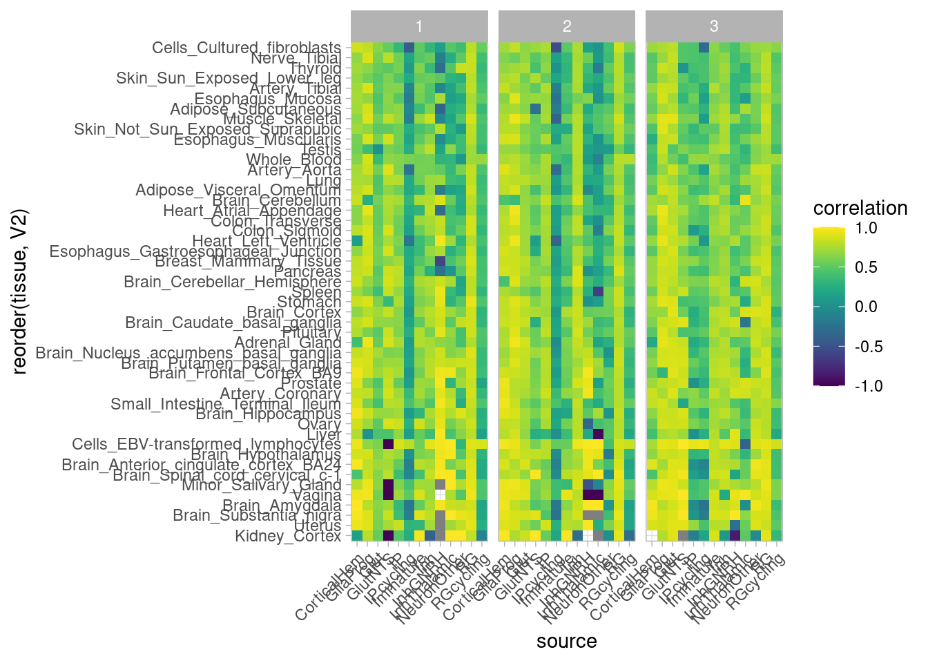

Finally, I do the same thing in a combined fashion so as to get an overall scatterplot (shown in Figure S5) and correlation, combining all tissues and conditions.

gtex_beta_snps_all <- list()

for (Y in gtex_names){
signif <- read.table(file = paste0("/project/gilad/umans/references/gtex/GTEx_Analysis_v8_eQTL/", Y), header = TRUE, sep = "\t", stringsAsFactors = FALSE) %>% filter(qval<0.05)

pairs <- read.table(file = paste0("/project/gilad/umans/references/gtex/GTEx_Analysis_v8_eQTL/", str_sub(Y, end=-14), "signif_variant_gene_pairs.txt.gz"), header = TRUE, sep = "\t", stringsAsFactors = FALSE)

joined <- pairs %>% select(variant_id, gene_id, slope, pval_nominal) %>% left_join(x=., y=signif %>% select(gene_id, gene_name), by=join_by( gene_id==gene_id), relationship="many-to-one") %>% 
  mutate(variant_id=str_sub(variant_id, start=4)) %>% 
  filter(str_detect(variant_id, "X_", negate = TRUE)) %>% #drop the X chromosome
  separate(variant_id, into = c("chrom", "position", "ref"), extra = "drop", sep="_", convert = TRUE) 
  
gtex_beta_snps_all[[Y]] <- inner_join(combined_all_snpgenes, joined, by=join_by(gene==gene_name, chrom==chrom, position==position), relationship="many-to-many") 

print(Y)
rm(signif, pairs, joined)
}

gtex_beta_snps_all <- readRDS(file = "/project2/gilad/umans/oxygen_eqtl/output/gtex_beta_snps_all.RDS")

gtex_beta_snps_all %>%  
  bind_rows(.id = "tissue") %>% 
  mutate(tissue=str_sub(tissue, end = -18)) %>% 
  ggplot(aes(x=beta, y=slope)) + geom_pointdensity(size=0.1) + scale_color_viridis() + theme_light() +
  xlab("Beta (organoid)") + ylab ("Beta (GTEx)") + geom_smooth(method="lm", linewidth=0.3, color="gray")

`geom_smooth()` using formula = 'y ~ x'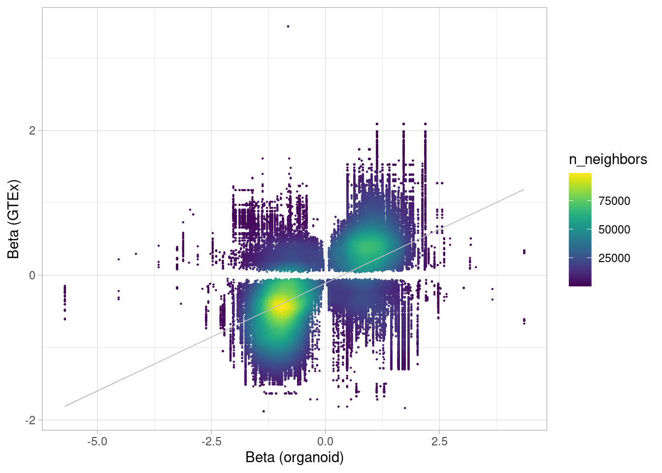

And to obtain an overall Pearson’s correlation and regression R^2:

a <- gtex_beta_snps_all %>%  
  bind_rows(.id = "tissue") %>% 
  mutate(tissue=str_sub(tissue, end = -18))
b <- lm(formula = slope ~ beta,  data =a)

summary(b)

Call:
lm(formula = slope ~ beta, data = a)

Residuals:
    Min      1Q  Median      3Q     Max 
-2.2431 -0.2928  0.0449  0.2866  3.7908 

Coefficients:
              Estimate Std. Error t value Pr(>|t|)    
(Intercept) -0.1094020  0.0008795  -124.4   <2e-16 ***
beta         0.2975402  0.0008201   362.8   <2e-16 ***
---
Signif. codes:  0 '***' 0.001 '**' 0.01 '*' 0.05 '.' 0.1 ' ' 1

Residual standard error: 0.5166 on 346494 degrees of freedom
Multiple R-squared:  0.2753,    Adjusted R-squared:  0.2753 
F-statistic: 1.316e+05 on 1 and 346494 DF,  p-value: < 2.2e-16

cor(a$beta, a$slope)

[1] 0.5247052

rm(a, b, gtex_beta_snps_all, gtex_beta_correlation_all_combined, combined_all_snpgenes, gtex_beta_correlation_all_plot, gtex_beta_recall)

Warning in rm(a, b, gtex_beta_snps_all, gtex_beta_correlation_all_combined, :
object 'gtex_beta_recall' not found

Compare to coarse-clustered results

mash_by_condition_output_coarse <- readRDS(file = "/project2/gilad/umans/oxygen_eqtl/output/combined_mash-by-condition_EE_coarse_reharmonized_newmash_032024.rds") %>% ungroup()  

mash_by_condition_output_coarse %>% 
  filter(sig_anywhere) %>% 
 mutate(class=case_when(control10_lfsr < 0.1 & allsharing ~ "class1",
                         control10_lfsr < 0.1 &  !allsharing ~ "class2",
                         sig_anywhere & control10_lfsr > 0.1 & !allsharing ~ "class3",
                         allsharing & control10_lfsr > 0.1 & (stim1pct_lfsr < 0.1 | stim21pct_lfsr < 0.1) ~ "class4")) %>%  group_by(source, class) %>% summarize(egenes=n()) %>% 
  ggplot(aes(x=factor(source, rev(coarse.order)), y=egenes, fill=factor(class, levels = c("class3", "class2", "class4", "class1"), ordered = TRUE))) + geom_bar(stat="identity") + 
  coord_flip() + theme_light() + theme(legend.title = element_blank()) + scale_fill_manual(values=class_colors) 

`summarise()` has grouped output by 'source'. You can override using the
`.groups` argument.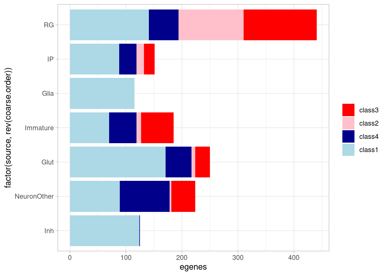

Past versions of unnamed-chunk-51-1.png

Version	Author	Date
f357871	Ben Umans	2025-02-24

Our hypothesis is that the the dynamic effects that emerge under treatment should be less represented in GTEx, compared to effects that are evident at baseline, as GTEx does not (explicitly) assess gene expression under different environmental perturbations (although post-mortem brain tissue may experience some amount of hypoxia and/or hyperoxia during sample collection). While not testing for sharing of regulatory sites or effects here, we can ask whether these dynamic eGenes are less likely to be present in GTEx compared to the dynamic eGenes present at baseline.

mash_by_condition_output_coarse %>% 
  filter(sig_anywhere) %>% 
  mutate(class=case_when(control10_lfsr < 0.1 & allsharing ~ "class1",
                         control10_lfsr < 0.1 &  !allsharing ~ "class2",
                         sig_anywhere & control10_lfsr > 0.1 & !allsharing ~ "class3",
                         sig_anywhere & allsharing ~ "class4")) %>%  #because of the order of assignment, this does not include "class1" egenes, ie those that are detectable under normoxia.  equivalent to `allsharing & control10_lfsr > 0.1 & (stim1pct_lfsr < 0.1 | stim21pct_lfsr < 0.1) ~ "class4"`
  group_by(source, class) %>% 
  summarise(egene_gtex = sum(gene %in% gtex_cortex_signif),
            egene_in_gtex_fraction = round((sum(gene %in% gtex_cortex_signif))/n(), 4)) %>% 
  ggplot(aes(x=factor(class, levels = c("class1", "class4", "class2", "class3")), y=egene_in_gtex_fraction)) + 
  geom_boxplot(outlier.shape = NA, aes(color=class), linewidth=0.4) + 
  geom_point(aes(group=source, color=source), position = position_jitter(width = 0.2, height = 0), size=0.5) + 
  xlab("eGene class (see note)") + 
  ylab("Fraction of eGenes in GTEx") + 
  theme_light() +  
  scale_color_manual(values=c(manual_palette_coarse, class_colors)) + theme(legend.position="none") 

`summarise()` has grouped output by 'source'. You can override using the
`.groups` argument.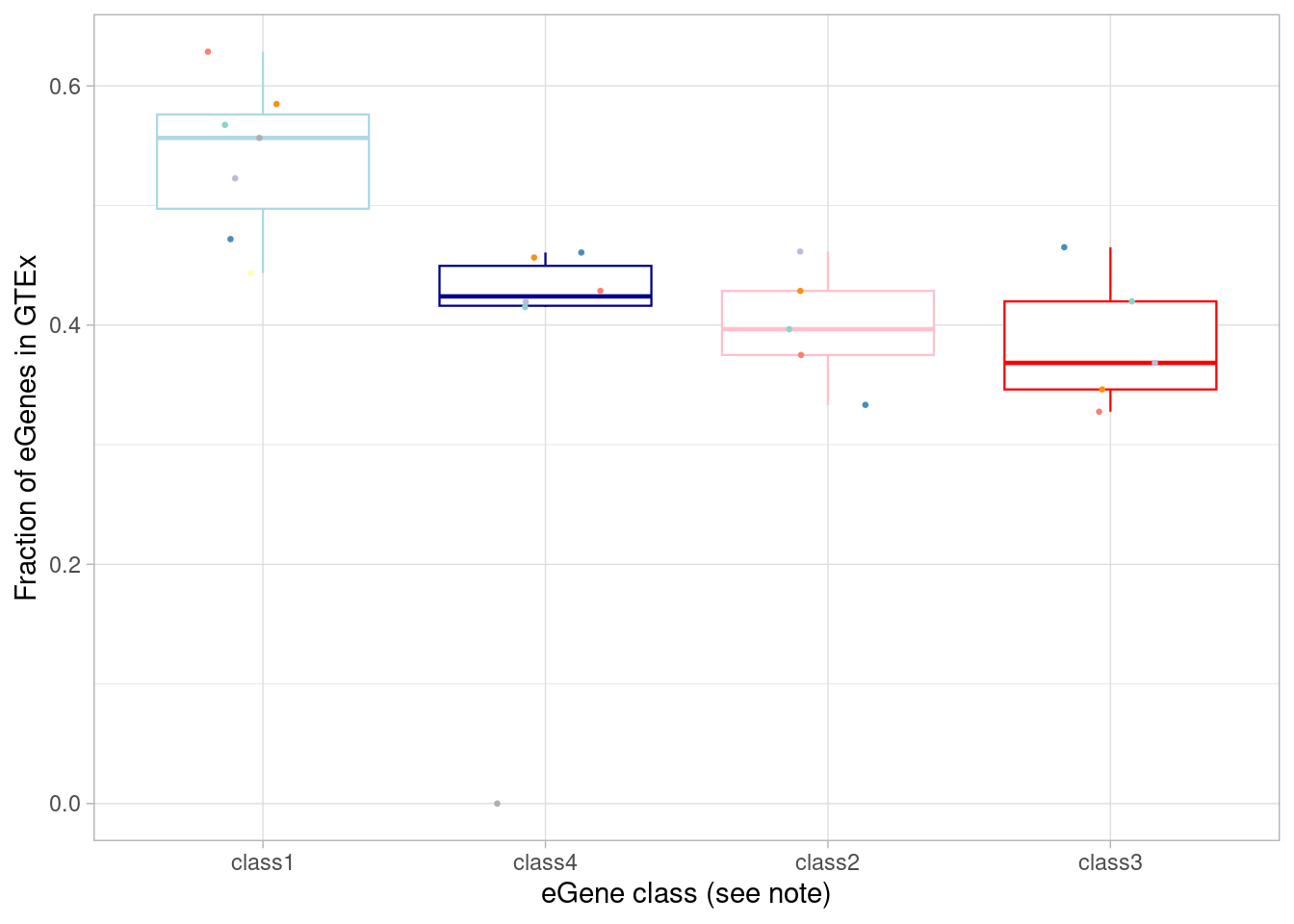

Past versions of unnamed-chunk-52-1.png

Version	Author	Date
f357871	Ben Umans	2025-02-24
f0eaf05	Ben Umans	2024-09-05

wilcox.test(mash_by_condition_output_coarse %>% 
  mutate(class=case_when(control10_lfsr < 0.1 & allsharing ~ "groupB",
                         control10_lfsr < 0.1 &  !allsharing ~ "groupB",
                         sig_anywhere & control10_lfsr > 0.1 & !allsharing ~ "groupA",
                         sig_anywhere & allsharing ~ "groupC", 
                         !sig_anywhere ~ "nonsig")) %>% 
    complete(source, class) %>% 
   group_by(source, class, .drop=FALSE) %>% 
    # filter(sig_anywhere) %>% 
  summarise(egene_gtex = sum(gene %in% (unlist(gtex_cortex_signif) %>% unique())),
            egene_in_gtex_fraction = (sum(gene %in% (unlist(gtex_cortex_signif) %>% unique())))/n()) %>% filter(class=="groupA") %>% pull(egene_in_gtex_fraction), 
  mash_by_condition_output_coarse %>% 
  filter(sig_anywhere) %>% 
  mutate(class=case_when(control10_lfsr < 0.1 & allsharing ~ "groupB",
                         control10_lfsr < 0.1 &  !allsharing ~ "groupB",
                         sig_anywhere & control10_lfsr > 0.1 & !allsharing ~ "groupA",
                         sig_anywhere & allsharing ~ "groupC")) %>% 
    complete(source, class) %>% 
   group_by(source, class, .drop=FALSE) %>% 
  summarise(egene_gtex = sum(gene %in% (unlist(gtex_cortex_signif) %>% unique())),
            egene_in_gtex_fraction = (sum(gene %in% (unlist(gtex_cortex_signif) %>% unique())))/n()) %>% filter(class %in% c("groupB")) %>% pull(egene_in_gtex_fraction), paired=TRUE,  alternative = "less")

`summarise()` has grouped output by 'source'. You can override using the
`.groups` argument.
`summarise()` has grouped output by 'source'. You can override using the
`.groups` argument.

    Wilcoxon signed rank exact test

data:  mash_by_condition_output_coarse %>% mutate(class = case_when(control10_lfsr < 0.1 & allsharing ~ "groupB", control10_lfsr < 0.1 & !allsharing ~ "groupB", sig_anywhere & control10_lfsr > 0.1 & !allsharing ~ "groupA", sig_anywhere & allsharing ~ "groupC", !sig_anywhere ~ "nonsig")) %>% complete(source, class) %>% group_by(source, class, .drop = FALSE) %>% summarise(egene_gtex = sum(gene %in% (unlist(gtex_cortex_signif) %>% unique())), egene_in_gtex_fraction = (sum(gene %in% (unlist(gtex_cortex_signif) %>%      unique())))/n()) %>% filter(class == "groupA") %>% pull(egene_in_gtex_fraction) and mash_by_condition_output_coarse %>% filter(sig_anywhere) %>% mutate(class = case_when(control10_lfsr < 0.1 & allsharing ~ "groupB", control10_lfsr < 0.1 & !allsharing ~ "groupB", sig_anywhere & control10_lfsr > 0.1 & !allsharing ~ "groupA", sig_anywhere & allsharing ~ "groupC")) %>% complete(source, class) %>% group_by(source, class, .drop = FALSE) %>% summarise(egene_gtex = sum(gene %in% (unlist(gtex_cortex_signif) %>% unique())), egene_in_gtex_fraction = (sum(gene %in% (unlist(gtex_cortex_signif) %>%      unique())))/n()) %>% filter(class %in% c("groupB")) %>% pull(egene_in_gtex_fraction)
V = 0, p-value = 0.007813
alternative hypothesis: true location shift is less than 0

The fraction of eGenes across cell types that would not be detected without treatment conditions is:

mash_by_condition_output_coarse %>% 
  filter(sig_anywhere) %>% 
  mutate(class=case_when(control10_lfsr < 0.1 & allsharing ~ "class1",
                         control10_lfsr < 0.1 &  !allsharing ~ "class2",
                         sig_anywhere & control10_lfsr > 0.1 & !allsharing ~ "class3",
                         allsharing & control10_lfsr > 0.1 & (stim1pct_lfsr < 0.1 | stim21pct_lfsr < 0.1) ~ "class4")) %>%  
  mutate(control_undetected=class %in% c("class3", "class4")) %>% 
  group_by(source) %>% 
  summarize(undetected_rate=sum(control_undetected)/n()) %>% 
  summarize(median(undetected_rate))

# A tibble: 1 × 1
  `median(undetected_rate)`
                      <dbl>
1                     0.331

The total number of eGenes detected here, in any condition or cell type, is:

mash_by_condition_output_coarse %>% 
  filter(sig_anywhere) %>% 
  pull(gene) %>% 
  unique() %>% 
  length()

[1] 1235

Many eGenes will have treatment-responsive effects in one cell type and treatment-shared effects in another cell type. The number of eGenes that have treatment-insensitive effects in at least one cell type is:

mash_by_condition_output_coarse %>% 
  filter(sig_anywhere) %>% 
  filter(allsharing) %>% 
  pull(gene) %>% 
  unique() %>% 
  length()

[1] 857

The number of eGenes that have treatment-sensitive effects in at least one cell type is:

mash_by_condition_output_coarse %>% 
  filter(sig_anywhere) %>% 
  filter(!allsharing) %>% 
  pull(gene) %>% 
  unique() %>% 
  length()

[1] 415

Calculate the number of “dynamic” vs “standard” eQTLs, here definesed by shared effect sizes.

mash_by_condition_output_coarse %>% 
  filter(sig_anywhere) %>% 
  group_by(source) %>% 
  summarize(allsharing=sum(allsharing), 
            total=n(), 
            hypox_normox=sum(hypoxia_normoxia_shared & sharing_contexts==1), 
            hyperox_normox=sum(hyperoxia_normoxia_shared & sharing_contexts==1), 
            treatment_shared=sum(hypoxia_hyperoxia_shared & sharing_contexts==1), 
            alldiff=sum(sharing_contexts==0), 
            associatively_shared=sum(sharing_contexts==2)) %>% 
  mutate(dynamic=total-allsharing) %>% 
  ungroup() %>% 
  summarise(across(allsharing:dynamic, median))

# A tibble: 1 × 8
  allsharing total hypox_normox hyperox_normox treatment_shared alldiff
       <int> <int>        <int>          <int>            <int>   <int>
1        125   185            6              2                2      18
# ℹ 2 more variables: associatively_shared <int>, dynamic <int>

Here, anything that does not have a similar (ie, within 2-fold) effect size in all three oxygen conditions is called “dynamic”. Within this dynamic category we can fine the following cases: * “treatment-shared” means different between normoxia and both hyperoxia and hypoxia, or, if you prefer, a normoxia-specific effect * “hypox_normox” means different in the hyperoxia condition from the other two * “hyperox_normox” means different in the hypoxia condition from the other two * “alldiff” means each oxygen condition has a different effect size from the other * “associatively_shared”, somewhat confusingly, means different between one pair of oxygen conditions but otherwise all shared. How can this happen? Consider a case where beta_normoxia=0.8, beta_hypoxia=0.4, and beta_hyperoxia=1.6. Here, both hypoxia and hyperoxia effects are shared with the normoxia condition (namely, differ by less than 2-fold), but differ from each other.

To plot these numbers:

class_colors3 <- c("allsharing"="blue", "partial_shared"="red", "normoxia_specific"="red", "hypoxia_specific"="red", "hyperoxia_specific"="red", "alldiff"="red")

p2 <- mash_by_condition_output_coarse %>% 
  filter(sig_anywhere) %>% 
 mutate(class=case_when(allsharing ~ "allsharing",
                        hypoxia_normoxia_shared & sharing_contexts==1 ~ "hyperoxia_specific",
                        hyperoxia_normoxia_shared & sharing_contexts==1 ~ "hypoxia_specific",
                        hypoxia_hyperoxia_shared & sharing_contexts==1 ~ "normoxia_specific",
                        sharing_contexts==2 ~ "partial_shared", 
                        sharing_contexts==0 ~ "alldiff"
                        )) %>%   #because of the order of assignment, this does not include "class1" egenes, ie those that are detectable under normoxia.  equivalent to `allsharing & control10_lfsr > 0.1 & (stim1pct_lfsr < 0.1 | stim21pct_lfsr < 0.1) ~ "class4"`
   group_by(source, class) %>% 
  summarise(egene = n()) %>% 
  ggplot(aes(x=factor(class, levels=c("allsharing", "alldiff", "normoxia_specific", "hypoxia_specific", "hyperoxia_specific",  "partial_shared"), ordered = TRUE), y=egene)) + 
  geom_boxplot(outlier.shape = NA, aes(color=class), linewidth=0.4) + 
  geom_point(aes(group=source, color=source), position = position_jitter(width = 0.2, height = 0), size=0.3) + 
  xlab("eGene class (see note)") + 
  ylab("Number of eGenes") + 
  theme_light() +  
  scale_color_manual(values=c(manual_palette_coarse, class_colors3)) + theme(legend.position="none") 

`summarise()` has grouped output by 'source'. You can override using the
`.groups` argument.

d2 <- mash_by_condition_output_coarse %>% 
  filter(sig_anywhere) %>% 
 mutate(class=case_when(allsharing ~ "allsharing",
                        hypoxia_normoxia_shared & sharing_contexts==1 ~ "hyperoxia_specific",
                        hyperoxia_normoxia_shared & sharing_contexts==1 ~ "hypoxia_specific",
                        hypoxia_hyperoxia_shared & sharing_contexts==1 ~ "normoxia_specific",
                        sharing_contexts==2 ~ "partial_shared", 
                        sharing_contexts==0 ~ "alldiff"
                        ),
        total=n(),
        standard=sum(allsharing)) %>%  
  mutate(dynamic=total-standard) %>% 
    group_by(class) %>% 
    summarise(egene = n(), total=median(total), standard=median(standard), dynamic=median(dynamic)) %>% 
    mutate(fraction_total=egene/total, fraction_dynamic=egene/dynamic) 

p2 + geom_point(aes(x=class, y=egene/5),  data = d2, shape=8, size=0.2) +
  scale_y_continuous(name = "eGenes per cell type", sec.axis = sec_axis(~ . *5, name="Total eQTLs"))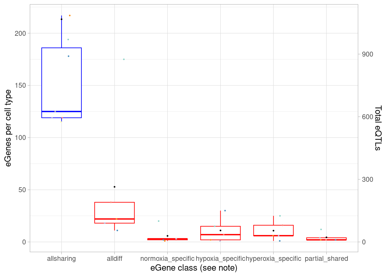 

What fraction of each of these categories are in GTEx?

mash_by_condition_output_coarse %>% 
  filter(sig_anywhere) %>% 
  mutate(class=case_when(allsharing ~ "allsharing",
                         hypoxia_normoxia_shared & sharing_contexts==1 ~ "hyperoxia_specific",
                         hyperoxia_normoxia_shared & sharing_contexts==1 ~ "hypoxia_specific",
                         hypoxia_hyperoxia_shared & sharing_contexts==1 ~ "normoxia_specific",
                         sharing_contexts==2 ~ "partial_shared", 
                         sharing_contexts==0 ~ "alldiff"
  )) %>%   #because of the order of assignment, this does not include "class1" egenes, ie those that are detectable under normoxia.  equivalent to `allsharing & control10_lfsr > 0.1 & (stim1pct_lfsr < 0.1 | stim21pct_lfsr < 0.1) ~ "class4"`
  group_by(source, class) %>% 
  summarise(egene_gtex = sum(gene %in% gtex_cortex_signif),
            egene_in_gtex_fraction = round((sum(gene %in% gtex_cortex_signif))/n(), 4)) %>% 
  ggplot(aes(x=factor(class, levels=c("allsharing", "partial_shared", "normoxia_specific", "hypoxia_specific", "hyperoxia_specific", "alldiff"), ordered = TRUE), y=egene_in_gtex_fraction)) + 
  geom_boxplot(outlier.shape = NA, aes(color=class), linewidth=0.4) + 
  geom_point(aes(group=source, color=source), position = position_jitter(width = 0.2, height = 0), size=0.5) + 
  xlab("eGene class (see note)") + 
  ylab("Fraction of eGenes in GTEx") + 
  theme_light() +  
  scale_color_manual(values=c(manual_palette_coarse, class_colors)) + theme(legend.position="none") 

`summarise()` has grouped output by 'source'. You can override using the
`.groups` argument.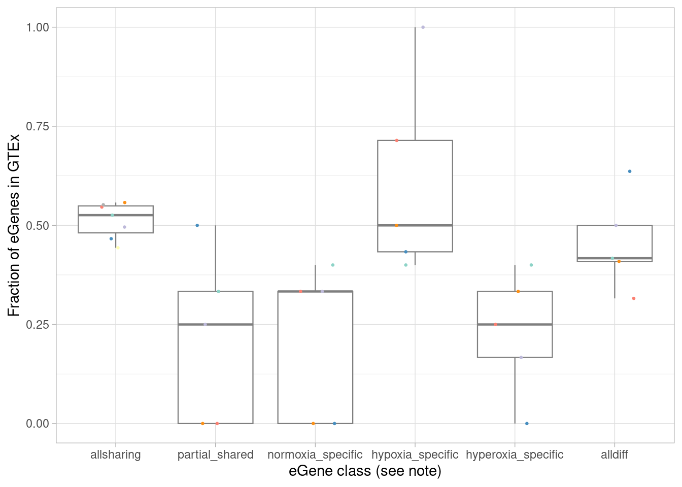

Past versions of unnamed-chunk-60-1.png

Version	Author	Date
f357871	Ben Umans	2025-02-24

We expect that the dynamic eGenes will be less represented in GTEx. To test this, I first designate the classes above as “standard” (all effects shared, or the strange case of all effects shared except for one comparison), or “dynamic”.

wilcox.test(mash_by_condition_output_coarse %>% 
 mutate(class=case_when(allsharing ~ "standard",
                        hypoxia_normoxia_shared & sharing_contexts==1 ~ "dynamic",
                        hyperoxia_normoxia_shared & sharing_contexts==1 ~ "dynamic",
                        hypoxia_hyperoxia_shared & sharing_contexts==1 ~ "dynamic",
                        sharing_contexts==2 ~ "standard", 
                        sharing_contexts==0 ~ "dynamic"
                        )) %>% 
   group_by(source, class, .drop = FALSE) %>% 
   filter(sig_anywhere) %>% 
   summarise(egene_gtex = sum(gene %in% (unlist(gtex_cortex_signif) %>% unique())),
            egene_in_gtex_fraction = (sum(gene %in% (unlist(gtex_cortex_signif) %>% unique())))/n()) %>%
   filter(class %in% c("dynamic")) %>% pull(egene_in_gtex_fraction), 
  mash_by_condition_output_coarse %>% 
  mutate(class=case_when(allsharing ~ "standard",
                        hypoxia_normoxia_shared & sharing_contexts==1 ~ "dynamic",
                        hyperoxia_normoxia_shared & sharing_contexts==1 ~ "dynamic",
                        hypoxia_hyperoxia_shared & sharing_contexts==1 ~ "dynamic",
                        sharing_contexts==2 ~ "standard", 
                        sharing_contexts==0 ~ "dynamic"
                        )) %>% 
   group_by(source, class, .drop = FALSE) %>% 
   filter(sig_anywhere) %>% 
  summarise(egene_gtex = sum(gene %in% (unlist(gtex_cortex_signif) %>% unique())),
            egene_in_gtex_fraction = (sum(gene %in% (unlist(gtex_cortex_signif) %>% unique())))/n()) %>%
   filter(class %in% c("standard")) %>% pull(egene_in_gtex_fraction), paired=TRUE, alternative = "less")

`summarise()` has grouped output by 'source'. You can override using the
`.groups` argument.
`summarise()` has grouped output by 'source'. You can override using the
`.groups` argument.

    Wilcoxon signed rank exact test

data:  mash_by_condition_output_coarse %>% mutate(class = case_when(allsharing ~ "standard", hypoxia_normoxia_shared & sharing_contexts == 1 ~ "dynamic", hyperoxia_normoxia_shared & sharing_contexts == 1 ~ "dynamic", hypoxia_hyperoxia_shared & sharing_contexts == 1 ~ "dynamic", sharing_contexts == 2 ~ "standard", sharing_contexts == 0 ~ "dynamic")) %>% group_by(source, class, .drop = FALSE) %>% filter(sig_anywhere) %>% summarise(egene_gtex = sum(gene %in% (unlist(gtex_cortex_signif) %>% unique())), egene_in_gtex_fraction = (sum(gene %in%      (unlist(gtex_cortex_signif) %>% unique())))/n()) %>% filter(class %in% c("dynamic")) %>% pull(egene_in_gtex_fraction) and mash_by_condition_output_coarse %>% mutate(class = case_when(allsharing ~ "standard", hypoxia_normoxia_shared & sharing_contexts == 1 ~ "dynamic", hyperoxia_normoxia_shared & sharing_contexts == 1 ~ "dynamic", hypoxia_hyperoxia_shared & sharing_contexts == 1 ~ "dynamic", sharing_contexts == 2 ~ "standard", sharing_contexts == 0 ~ "dynamic")) %>% group_by(source, class, .drop = FALSE) %>% filter(sig_anywhere) %>% summarise(egene_gtex = sum(gene %in% (unlist(gtex_cortex_signif) %>% unique())), egene_in_gtex_fraction = (sum(gene %in%      (unlist(gtex_cortex_signif) %>% unique())))/n()) %>% filter(class %in% c("standard")) %>% pull(egene_in_gtex_fraction)
V = 0, p-value = 0.03125
alternative hypothesis: true location shift is less than 0

Topic analysis

Here, I outline the steps used to fit a 15-topic model to our data and then estimate topic-interacting QTLs using CellRegMap.

First, cluster at high resolution to obtain pseudocells, which are defined by individual and treatment.

harmony.batchandindividual.sct <- readRDS(file = "/project2/gilad/umans/oxygen_eqtl/output/harmony_organoid_dataset.rds")
subset_seurat <- subset(harmony.batchandindividual.sct, subset = vireo.prob.singlet > 0.95 & nCount_RNA<20000 & nCount_RNA>2500 & treatment != "control21")

subset_seurat$splitkey <- paste0(subset_seurat$treatment, "_", subset_seurat$vireo.individual)
subset_seurat <- FindNeighbors(object = subset_seurat, reduction = "harmony", dims = 1:100, verbose = TRUE)

Computing nearest neighbor graph

Computing SNN

subset_seurat <- FindClusters(object = subset_seurat, dims = 1:100, resolution = 20)

Warning: The following arguments are not used: dims

Warning: The following arguments are not used: dims

Modularity Optimizer version 1.3.0 by Ludo Waltman and Nees Jan van Eck

Number of nodes: 170841
Number of edges: 6947030

Running Louvain algorithm...
Maximum modularity in 10 random starts: 0.6973
Number of communities: 258
Elapsed time: 94 seconds

2 singletons identified. 256 final clusters.

subset_seurat$pseudocell <- paste0(subset_seurat$splitkey, "_", subset_seurat$seurat_clusters)

Then, obtain pseudobulk data from the pseudocells.

pseudocell_pseudobulk <- generate.pseudobulk(subset_seurat, labels = "pseudocell")
saveRDS(pseudocell_pseudobulk, file = "output/pseudocell_pseudobulk_nocontrol21_032024.RDS")

Next, compile the metadata for the pseudocells, which CellRegMap will need:

a <- subset_seurat@meta.data %>% 
  select(pseudocell, donor_id=vireo.individual, sex, treatment) %>%
  distinct() %>% 
  remove_rownames() %>% 
  column_to_rownames(var = "pseudocell")

treatment <- model.matrix(~ -1 +  treatment, data=a)
sex <- model.matrix(~-1 +  sex, data=a)

metadata_output <- bind_cols(a, treatment, sex) %>% 
  rownames_to_column(var = "pseudocell") %>% 
  select(pseudocell, donor_id, treatmentcontrol10, treatmentstim1pct, treatmentstim21pct, sexfemale) %>% 
  arrange(pseudocell)

write_tsv(metadata_output, file = "topicqtl/pseudocell_metadata_r20_harmonized.tsv")

For CellRegMap, we need normalized counts. Per guidance from the Battle Lab (JHU), we use the PFlog1pPF method from this paper, but instead of using means for the PF we use the median. It works by multiplying the read counts in each pseudocell by the ratio of median(read depth over all pseudocells)/that cell’s read depth. So, we do that on the pseudobulk counts, then take log1p of those, then do it again.

counts <- t(pseudocell_pseudobulk$counts)

first_median <- median(rowSums(counts))
first_pf <- t(apply(X = counts, MARGIN = 1, FUN = function(x) x*(first_median/sum(x))))
first_pf_log1p <- log1p(first_pf)

second_median <- median(rowSums(first_pf_log1p))
second_pf <- t(apply(X = first_pf_log1p, MARGIN = 1, FUN = function(x) x*(second_median/sum(x))))

for_crm <- as.data.frame(second_pf) %>% 
  rownames_to_column("names") %>% 
  arrange(names) %>% 
  column_to_rownames("names")

write.table(for_crm, file = "/project2/gilad/umans/oxygen_eqtl/output/topics_pseudocell_counts_nocontrol21_normalized.tsv", quote = FALSE, sep = "\t", row.names = TRUE, col.names = TRUE)

Fit topic model

Next, we fit a 15-topic model using fastTopics.

library(fastTopics)

Remove genes with very low expression:

j <- which(colSums(counts)>40)
counts <- counts[,j]

fit <- fit_poisson_nmf(counts, k = 15, init.method = "random", 
                       method = "em", numiter = 400, control = list(nc = 10, numiter = 4), 
                       verbose = c("detailed"))

fit <- fit_poisson_nmf(counts, fit0 = fit, method = "scd", numiter = 200,
                       control = list(numiter = 4, nc = 10, extrapolate = TRUE),
                       verbose = c("detailed"))

fit <- poisson2multinom(fit)

as_tibble(fit$L, rownames="pseudocell") %>%
  arrange(pseudocell) %>% 
  write_tsv(file = "topicqtl/pseudocell_loadings_k15.tsv")

Plot the topic loadings by cell type and treatment condition:

annotations <- subset_seurat@meta.data %>% group_by(pseudocell) %>%
  summarise(individual=names(which.max(table(vireo.individual))),
            treatment=names(which.max(table(treatment))),
            coarse=names(which.max(table(combined.annotation.coarse.harmony))),
            fine=names(which.max(table(combined.annotation.fine.harmony)))) 

coarse_labels <- enframe(annotations %>% pull(coarse, name=pseudocell), name = "pseudocell", value = "coarse")
fine_labels <- enframe(annotations %>% pull(fine, name=pseudocell), name = "pseudocell", value = "fine")
treatment_labels <- enframe(annotations %>% pull(treatment, name=pseudocell), name = "pseudocell", value = "treatment")
individual_labels <- enframe(annotations %>% pull(individual, name=pseudocell), name = "pseudocell", value = "individual")

fit <- readRDS(file = "/project2/gilad/umans/oxygen_eqtl/output/topics_pseudocells_15_nocontrol21_20240124.RDS")

plot.data <- as.data.frame(fit$L) %>% 
  rownames_to_column(var = "pseudocell") %>% 
  pivot_longer(cols = !pseudocell, names_to = "topic", values_to = "loading") %>% 
  left_join(y= coarse_labels) %>% 
  left_join(y= fine_labels) %>% 
  left_join(y= treatment_labels) %>% 
  left_join(y= individual_labels) %>% 
  group_by(fine, treatment, topic) %>% 
  summarise(plot_value=mean(loading)) %>% 
  pivot_wider(values_from = plot_value, names_from = topic) %>% 
  unite(col = "rowname", fine:treatment, sep = "_") %>% 
  column_to_rownames(var = "rowname") %>% 
  as.matrix()

Joining with `by = join_by(pseudocell)`
Joining with `by = join_by(pseudocell)`
Joining with `by = join_by(pseudocell)`
Joining with `by = join_by(pseudocell)`
`summarise()` has grouped output by 'fine', 'treatment'. You can override using
the `.groups` argument.

labels <- data.frame(fine=str_extract(rownames(plot.data), pattern = "[^_]+"),
                     treatment=str_extract(rownames(plot.data), pattern = "[^_]+$")
                     )
rownames(labels) <- rownames(plot.data)

celltypeCol <- manual_palette_fine

treatmentCol <- c("control10" = "gray", "stim1pct" = "blue", "stim21pct"="red")
annoCol <- list(fine = celltypeCol,
                treatment = treatmentCol)

# now use pheatmap to annotate
labels$fine <- factor(labels$fine, levels = c("RGcycling" , "RG",  "CorticalHem",  "IPcycling", "IP", "GliaProg", "Oligo", "Immature", "Glut", "GlutNTS", "NeuronOther",  "MidbrainDA", "Cajal", "Inh",  "InhThalamic", "InhGNRH",  "InhSST", "InhMidbrain",  "Choroid", "VLMC"))

sub_samp_ordered <- plot.data[rownames(arrange(labels, fine)), c("k7", "k1", "k2",  "k3",  "k4", "k5", "k6",  "k8", "k9", "k10", "k11", "k12", "k13", "k14", "k15")  ]
# sub_samp_ordered <- plot.data[rownames(arrange(labels, treatment, fine)), ]

pheatmap(sub_samp_ordered, col = colorRampPalette(rev(brewer.pal(11, "Spectral")))(25),
         border_color = NA,
         show_colnames = TRUE,
         treeheight_row = 0, treeheight_col = 0,
         annotation_row = labels, 
         annotation_colors = annoCol,
         cluster_rows = FALSE, cluster_cols = FALSE
         )

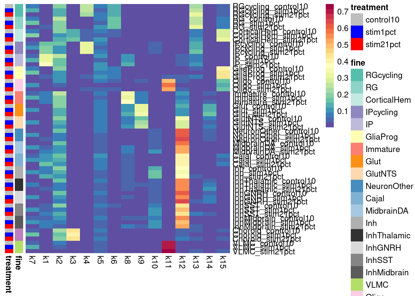
Topic model DE

Next, I used the grade of membership differential expression routine in fastTopics to compare marker genes for hypoxia-associated topoic 7 with the hypoxia genes we used for responsive cell identification.

de_output <- de_analysis(fit, counts, pseudocount = 0.1,
                  control = list(ns = 1e4, nc = 10), shrink.method="ash", verbose=TRUE)

de_15 <- readRDS(file = "/project2/gilad/umans/oxygen_eqtl/output/topics_pseudocells_15_de_output_20240124.RDS")

mash.hypoxia <- c("BNIP3", "IGFBP2", "PGAM1", "BNIP3L", 
  "FAM162A", "TPI1", "PGK1", "P4HA1", 
  "ENO1",  "LDHA", "MIR210HG", "ALDOA", 
  "AC097534.2", "MTFP1", "AK4", "SLC2A1",
  "VEGFA", "PDK1", "RCOR2", "ANKRD37",
  "PLOD2", "HK2", "TNIP1", "DDIT4", "AC107021.1",
  "INSIG2", "WSB1", "NRN1", "PPFIA4", "EGLN1", 
  "RAPGEF4", "FAM210A", "P4HA2", "CXCR4", 
  "GOLGA8A", "ENO2", "SNHG19", "GPI", "HLA-B",
  "MT3", "ADAMTS20", "PFKP", "PFKFB3", "HILPDA", 
  "KDM3A", "RLF", "KDM7A", "AC087280.2", "HK1", 
  "HIF1A-AS3", "PDK3", "LINC02649", "FUT11", 
  "NIM1K", "COL11A1", "AL357153.2", "KDM4C", 
  "UACA", "SLC16A1", "USP28", "SLC8A3", 
  "RASGRF1", "NRIP3", "PRMT8", "NDRG1", "PCAT6", "RAPGEF4-AS1")

plot_data <- data.frame(logfc=de_15$postmean[,"k7"], z=abs(de_15$z[,"k7"]), lfsr=de_15$lfsr[,"k7"])
plot_data$mark <- "black"
plot_data[which(plot_data$lfsr > 0.05 ), "mark"] <- "lightgray"
plot_data[which(rownames(plot_data) %in% mash.hypoxia), "mark"] <- "red"

hypoxia_points <- plot_data[which(plot_data$mark %in% c("black", "lightgray")),]
highlight_points <- plot_data[which(plot_data$mark %in% c("red")),]

ggplot(data=hypoxia_points, aes(x=logfc, y=z, color=mark,  label=rownames(hypoxia_points)) ) + 
  geom_point( alpha=0.5, size=0.2)  +
  scale_color_identity() + 
  scale_y_continuous(trans = "sqrt") + theme_light() +
  geom_point(data=highlight_points, aes(x=logfc, y=z, color=mark, label=rownames(highlight_points)), size=0.2) + 
  geom_text_repel(data = highlight_points, aes(x=logfc, y=z, color=mark, label=rownames(highlight_points)), size=1.8, color="black") + 
  ggtitle("topic 7")

Warning in geom_point(data = highlight_points, aes(x = logfc, y = z, color =
mark, : Ignoring unknown aesthetics: label

Warning: Removed 208 rows containing missing values (`geom_point()`).

Warning: ggrepel: 19 unlabeled data points (too many overlaps). Consider
increasing max.overlaps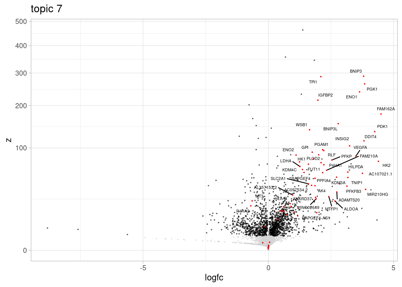

Past versions of unnamed-chunk-72-1.png

Version	Author	Date
d3c2181	Ben Umans	2025-02-25
f357871	Ben Umans	2025-02-24

I do the same for topic 4, which marks dividing cells, using markers of dividing cells that we see in the pseudobulk data

plot_data <- data.frame(logfc=de_15$postmean[,"k4"], z=abs(de_15$z[,"k4"]), lfsr=de_15$lfsr[,"k4"])
plot_data$mark <- "black"
plot_data[which(plot_data$lfsr > 0.05 ), "mark"] <- "lightgray"
plot_data[which(rownames(plot_data) %in% c("MKI67", "TOP2A", "CDCA8", "CDCA3", "CENPE", "CDC20", "CDCA2", "CDC25C", "CCNA2", "CEP55", "CENPF")), "mark"] <- "red"

plot_points <- plot_data[which(plot_data$mark %in% c("black", "lightgray")),]
highlight_points <- plot_data[which(plot_data$mark %in% c("red")),]

ggplot(data=plot_points %>% filter(z<300), aes(x=logfc, y=z, color=mark,  label=rownames(plot_points %>% filter(z<300))) ) + 
  geom_point( alpha=0.5, size=0.2)  + 
  scale_color_identity()  + 
  theme_light() + 
  geom_point(data=highlight_points, aes(x=logfc, y=z, color=mark, label=rownames(highlight_points)), size=0.2) + geom_text_repel(data = highlight_points, aes(x=logfc, y=z, color=mark, label=rownames(highlight_points)), color="black", size=1.8)   + scale_y_continuous(trans = "sqrt") +
  ggtitle("topic 4")

Warning in geom_point(data = highlight_points, aes(x = logfc, y = z, color =
mark, : Ignoring unknown aesthetics: label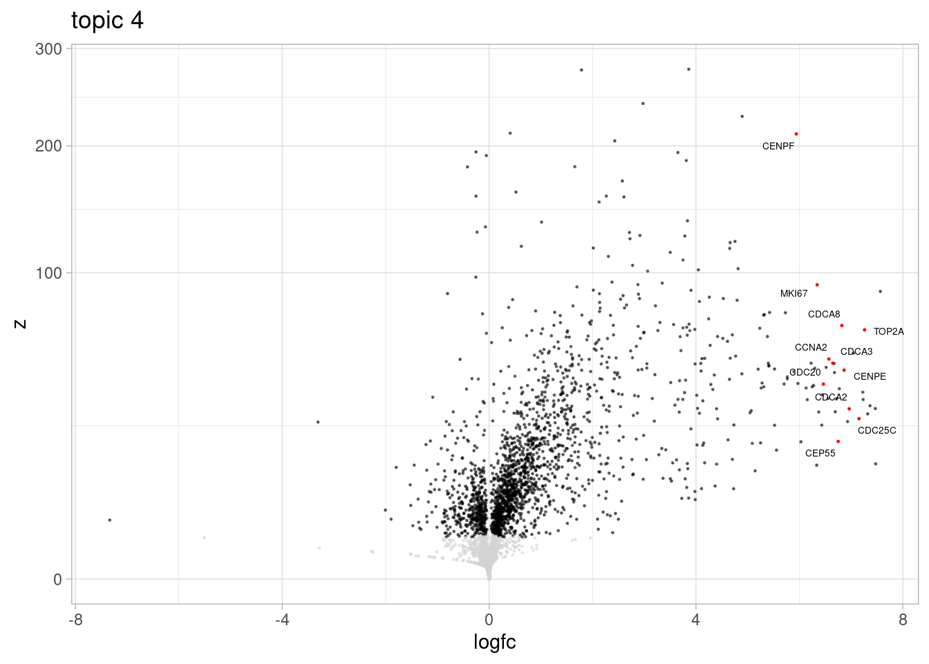

Past versions of unnamed-chunk-73-1.png

Version	Author	Date
d3c2181	Ben Umans	2025-02-25

And the same for cortical hem-associated topic 3

plot_data_hem <- data.frame(logfc=de_15$postmean[,"k3"], z=abs(de_15$z[,"k3"]), lfsr=de_15$lfsr[,"k3"])
plot_data_hem$mark <- "black"
plot_data_hem[which(plot_data_hem$lfsr > 0.05 ), "mark"] <- "lightgray"
plot_data_hem[which(rownames(plot_data_hem) %in% c("WLS", "WNT2B", "WNT5A",  "WNT8B", "RSPO1", "RSPO2",   "TTR" , "CLIC6", "FOLR1")), "mark"] <- "red"

hem_points <- plot_data_hem[which(plot_data_hem$mark %in% c("black", "lightgray")),]
highlight_points <- plot_data_hem[which(plot_data_hem$mark %in% c("red")),]

ggplot(data=hem_points, aes(x=logfc, y=z, color=mark,  label=rownames(hem_points)) ) + 
  geom_point( alpha=0.5, size=0.2)  + 
  scale_color_identity() + 
  scale_y_continuous(trans = "sqrt") + 
  theme_light() +  
  geom_point(data=highlight_points, aes(x=logfc, y=z, color=mark, label=rownames(highlight_points)), size=0.2) + 
  geom_text_repel(data = highlight_points, aes(x=logfc, y=z, color=mark, label=rownames(highlight_points)), size=1.8,  color="black") + 
  ggtitle("topic 3")

Warning in geom_point(data = highlight_points, aes(x = logfc, y = z, color =
mark, : Ignoring unknown aesthetics: label

Warning: Removed 343 rows containing missing values (`geom_point()`).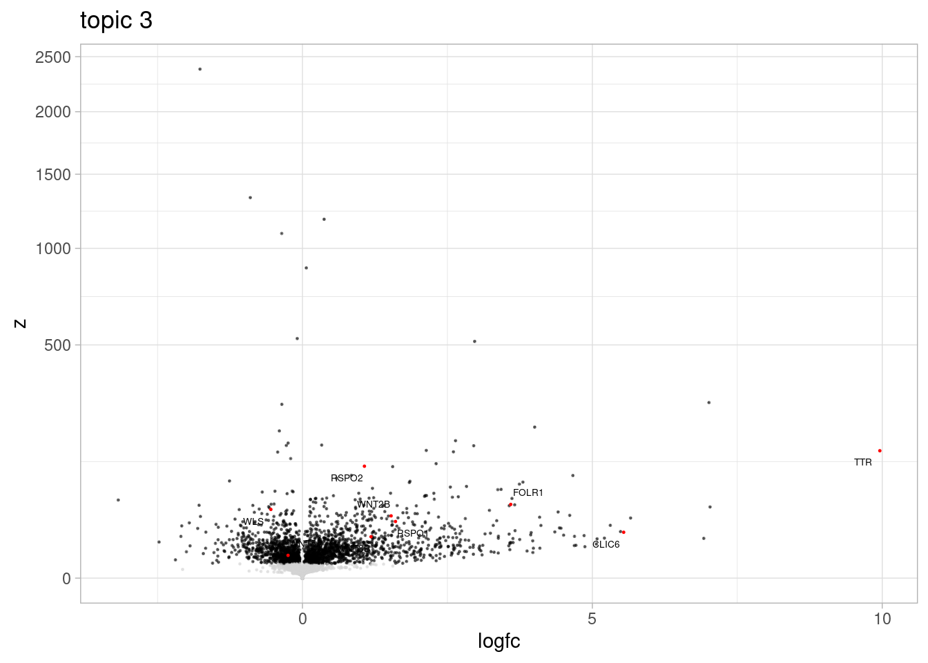

Past versions of unnamed-chunk-74-1.png

Version	Author	Date
d3c2181	Ben Umans	2025-02-25
f357871	Ben Umans	2025-02-24

Prepare CellRegMap input

Interaction testing with CellRegMap works on a subset of SNP-gene pairs, as it is computationally costly to do a true genome-wide scan. However, there is no guarantee that the lead SNP chosen by mash’s fastqtl2mash procedure is the uniquely best SNP to test in all pseudocells. I therefore go back to the MatrixEQTL output and, for each eGene/cell type/condition, retain all eQTL SNPs with equivalent or better evidence of association as the mash SNP.

controlset <- mash_by_condition_output %>% 
  filter(control10_lfsr<0.1) %>% 
  separate(gene_snp, into = c("genename", "snp"), sep = "_") %>% 
  # mutate(snp = str_sub(snp, end = -5)) %>% 
  select(snp, gene, source, control10_lfsr)
  
control_all_snps <- lapply(as.character(unique(controlset$source)), function(x) 
  controlset %>% filter(source==x) %>% #go cell type by cell type
    full_join(y=read.table(paste0("/project2/gilad/umans/oxygen_eqtl/data/MatrixEQTL/output/combined_fine_quality_filter20_032024/results_combined_control10_", x,"_nominal.txt"), head=TRUE, stringsAsFactors=FALSE), by=join_by(gene, snp==snps)) %>% #join with original snp-gene pairs form which mash drew
    dplyr::filter(gene %in% (controlset %>% filter(source==x) %>% pull(gene))) %>% #filter to only those genes for which mash found a significant eqtl
    mutate(control10_lfsr=replace_na(control10_lfsr, replace = 0)) %>% #there will be a lfsr for only the mash lead variant.  set all others to 0
    group_by(gene) %>% 
    arrange(pvalue, control10_lfsr, .by_group = TRUE) %>% #first sort by ascending pvalue, then ascending lfsr. because we set the others to 0, this ensures we sort such that the mash lead variant comes last
    dplyr::slice(1:match(TRUE, !is.na(source))) %>% #take all of the snp-gene pairs up to the mash-chosen one
    select(snp, gene) %>% 
    mutate(source=x)
  ) %>% bind_rows() %>% distinct()

hypoxiaset <- mash_by_condition_output %>% 
  filter(stim1pct_lfsr < 0.1) %>% 
  separate(gene_snp, into = c("genename", "snp"), sep = "_") %>% 
  # mutate(snp = str_sub(snp, end = -5)) %>% 
  select(snp, gene, source, stim1pct_lfsr)

hypoxia_all_snps <- lapply(as.character(unique(hypoxiaset$source)), function(x) 
  hypoxiaset %>% filter(source==x) %>% full_join(y=read.table(paste0("/project2/gilad/umans/oxygen_eqtl/data/MatrixEQTL/output/combined_fine_quality_filter20_032024/results_combined_stim1pct_", x,"_nominal.txt"), head=TRUE, stringsAsFactors=FALSE), by=join_by(gene, snp==snps)) %>% 
    dplyr::filter(gene %in% (hypoxiaset %>% filter(source==x) %>% pull(gene))) %>% 
    mutate(stim1pct_lfsr=replace_na(stim1pct_lfsr, replace = 0)) %>% 
    group_by(gene) %>% 
    arrange(pvalue, stim1pct_lfsr, .by_group = TRUE) %>% 
    dplyr::slice(1:match(TRUE, !is.na(source))) %>% 
    select(snp, gene) %>% 
    mutate(source=x)
  ) %>% bind_rows() %>% distinct()

hyperoxiaset <- mash_by_condition_output %>% 
  filter(stim21pct_lfsr < 0.1) %>% 
  separate(gene_snp, into = c("genename", "snp"), sep = "_") %>% 
  # mutate(snp = str_sub(snp, end = -5)) %>% 
  select(snp, gene, source, stim21pct_lfsr)

hyperoxia_all_snps <- lapply(as.character(unique(hyperoxiaset$source)), function(x) 
  hyperoxiaset %>% filter(source==x) %>% full_join(y=read.table(paste0("/project2/gilad/umans/oxygen_eqtl/data/MatrixEQTL/output/combined_fine_quality_filter20_032024/results_combined_stim21pct_", x,"_nominal.txt"), head=TRUE, stringsAsFactors=FALSE), by=join_by(gene, snp==snps)) %>% 
    dplyr::filter(gene %in% (hyperoxiaset %>% filter(source==x) %>% pull(gene))) %>% 
    mutate(stim21pct_lfsr=replace_na(stim21pct_lfsr, replace = 0)) %>% 
    group_by(gene) %>% 
    arrange(pvalue, stim21pct_lfsr, .by_group = TRUE) %>% 
    dplyr::slice(1:match(TRUE, !is.na(source))) %>% 
    select(snp, gene) %>% 
    mutate(source=x)
  ) %>% bind_rows() %>% distinct()

bind_rows(control_all_snps, hypoxia_all_snps, hyperoxia_all_snps) %>% ungroup() %>% 
  distinct() %>%
  write_tsv(file = "/project2/gilad/umans/oxygen_eqtl/data/MatrixEQTL/output/combined_fine_quality_filter20_032024/mash/post-mash_significant_and_equivalent_snp-gene_pairs_EE.txt", col_names = FALSE)

Then use these SNP-gene pairs, with some minor reformatting for CellRegMap:

snpgenes <- read_tsv(file = "/project2/gilad/umans/oxygen_eqtl/data/MatrixEQTL/output/combined_fine_quality_filter20_032024/mash/post-mash_significant_and_equivalent_snp-gene_pairs_EE.txt", col_names = c("snp", "gene", "source"))

snpgenes %>% mutate(mutated=str_extract(snp, pattern = "[:digit:]+:[:digit:]+")) %>% 
  separate_wider_delim(mutated, delim = ":", names = c("chrom", "END")) %>% 
  mutate(END=as.integer(END)) %>% 
  mutate(`#CHR`=paste0("chr", chrom)) %>% 
  mutate(START= END - 1) %>% 
  select(`#CHR`, START, END, GENE_ENSG=gene, GENE_HGNC=gene, VARIANT_ID=snp, CELLTYPE=source) %>% 
  write_tsv(file = "/project2/gilad/umans/oxygen_eqtl/topicqtl/mash_and_equivalent_fine_reharmonized.bed")

Metadata for CellRegMap was extracted from the pseudocell data as follows:

a <- subset_seurat@meta.data %>% select(pseudocell, donor_id=vireo.individual, sex, treatment) %>% distinct() %>% remove_rownames() %>%  column_to_rownames(var = "pseudocell")

treatment <- model.matrix(~-1 +  treatment, data=a)
sex <- model.matrix(~-1 +  sex, data=a)

metadata_output <- bind_cols(a, treatment, sex) %>% 
  rownames_to_column(var = "pseudocell") %>% 
  select(pseudocell, donor_id, treatmentcontrol10, treatmentstim1pct, treatmentstim21pct, sexfemale) %>% 
  arrange(pseudocell)

write_tsv(metadata_output, file = "topicqtl/pseudocell_metadata_r20_harmonized.tsv")

Run CellRegMap

CellRegMap was run using the Snakemake rule cellregmap_eqtl_calling.py with accompanying code in code/cellregmap_eqtl_calling/.

Process CellRegMap output

After Bonferroni correction and determination of a q-value threshold, we obtain the significant CellRegMap output. To identify QTL effects correlated with particular topics, I first calculate the correlation between the estimated effect sizes for each pseudocell and the topic loadings for that pseudocell.

crm_signif <- vroom("/project2/gilad/umans/oxygen_eqtl/topicqtl/outputs/topics15/all_genes_merged_fine_fasttopics_15_topics.cellregmap.sighits.tsv")

Rows: 289 Columns: 5
── Column specification ────────────────────────────────────────────────────────
Delimiter: "\t"
chr (2): GENE_HGNC, VARIANT_ID
dbl (3): P_CELLREGMAP, P_BONF, q

ℹ Use `spec()` to retrieve the full column specification for this data.
ℹ Specify the column types or set `show_col_types = FALSE` to quiet this message.

crm_iegenes <- crm_signif$GENE_HGNC

crm_betas <- vroom(paste0("/project2/gilad/umans/oxygen_eqtl/topicqtl/outputs/topics15/fasttopics_fine_15_topics.", crm_iegenes, ".cellregmap.betas.tsv"))

Rows: 3094323 Columns: 5
── Column specification ────────────────────────────────────────────────────────
Delimiter: "\t"
chr (3): PSEUDOCELL, GENE_HGNC, VARIANT_ID
dbl (2): BETA_GXC, BETA_G

ℹ Use `spec()` to retrieve the full column specification for this data.
ℹ Specify the column types or set `show_col_types = FALSE` to quiet this message.

crm_betas_wide <- dplyr::select(crm_betas, c(PSEUDOCELL, BETA_GXC, GENE_HGNC, VARIANT_ID)) %>%
  unite(TOPIC_QTL, GENE_HGNC, VARIANT_ID, sep="_") %>%
  pivot_wider(id_cols=PSEUDOCELL, names_from=TOPIC_QTL, values_from=BETA_GXC)

topic_loadings <- vroom("/project2/gilad/umans/oxygen_eqtl/topicqtl/pseudocell_loadings_k15.tsv")

Rows: 10707 Columns: 16
── Column specification ────────────────────────────────────────────────────────
Delimiter: "\t"
chr  (1): pseudocell
dbl (15): k1, k2, k3, k4, k5, k6, k7, k8, k9, k10, k11, k12, k13, k14, k15

ℹ Use `spec()` to retrieve the full column specification for this data.
ℹ Specify the column types or set `show_col_types = FALSE` to quiet this message.

crm_betas_loadings <- left_join(crm_betas_wide, topic_loadings, by=c("PSEUDOCELL"="pseudocell"))

beta_topic_corrs_matrix <- cor(dplyr::select(crm_betas_loadings, -c(PSEUDOCELL, paste0("k", seq(15)))),
                        dplyr::select(crm_betas_loadings, paste0("k", seq(15))))

Export as a table for supplement:

data.frame(beta_topic_corrs_matrix) %>% rownames_to_column(var="Gene-SNP") %>%  write_csv(file = "docs/STable_CRM.csv")

How many of these topic 7-interacting QTLs are not detected as dynamic in the static analysis?

beta_topic_corrs_p <- apply(dplyr::select(crm_betas_loadings, -c(PSEUDOCELL, paste0("k", seq(15)))) %>% as.matrix(), MARGIN = 2, FUN = function(x) cor.test(x, crm_betas_loadings$k7)$p.value )

beta_topic_corrs_matrix %>% as.data.frame() %>% 
  dplyr::select(k7) %>% 
  bind_cols(pval=beta_topic_corrs_p) %>% 
  rownames_to_column(var = "gene_snp") %>%  
   separate(gene_snp, into = c("genename", "snp"), sep = "_") %>% 
    mutate(snp_short = str_sub(snp, end = -5)) %>% 
  filter(pval < (0.05/289)) %>% dim()

[1] 218   5

# Many of these have small correlations with k7, which are nonetheless statistically significant.  How many if we threshold to correlation coefficient > 0.1?
beta_topic_corrs_matrix %>% as.data.frame() %>% 
  dplyr::select(k7) %>% 
  bind_cols(pval=beta_topic_corrs_p) %>% 
  rownames_to_column(var = "gene_snp") %>%  
   separate(gene_snp, into = c("genename", "snp"), sep = "_") %>% 
    mutate(snp_short = str_sub(snp, end = -5)) %>% 
  filter(pval < (0.05/289)) %>% filter(k7>0.1) %>% dim()

[1] 58  5

k7_egenes <- beta_topic_corrs_matrix %>% as.data.frame() %>% 
  dplyr::select(k7) %>% 
  bind_cols(pval=beta_topic_corrs_p) %>% 
  rownames_to_column(var = "gene_snp") %>%  
   separate(gene_snp, into = c("genename", "snp"), sep = "_") %>% 
    mutate(snp_short = str_sub(snp, end = -5)) %>% 
  filter(pval < (0.05/289)) %>% filter(k7>0.1) %>% pull(genename)

How many of these are more strongly correlated with k7 than any other topic?

beta_topic_corrs_matrix %>% as.data.frame() %>% 
  bind_cols(pval=beta_topic_corrs_p) %>% 
  rownames_to_column(var = "gene_snp") %>%  
   separate(gene_snp, into = c("genename", "snp"), sep = "_") %>% 
    mutate(snp_short = str_sub(snp, end = -5)) %>% 
  mutate(max=pmax(abs(k1), abs(k2), abs(k3), abs(k4), abs(k5), abs(k6), abs(k7), abs(k8), abs(k9), abs(k10), abs(k11), abs(k12), abs(k13), abs(k14), abs(k15))) %>% 
  filter(pval < (0.05/289)) %>% arrange(desc(abs(k7))) %>% 
  filter(abs(k7)==max)

  genename             snp         k1         k2        k3          k4
1   WDR45B 17:82613559:C:G -0.4762630 -0.2143771 0.3363079  0.21655061
2   CRABP2 1:156697607:C:T -0.4175295  0.2197124 0.1105780 -0.04775569
          k5         k6        k7         k8         k9         k10        k11
1 -0.1933042  0.3782810 0.6479771 -0.5483449 -0.1040422 -0.04133576 0.28243572
2 -0.1547579 -0.2154844 0.4939605 -0.4480681 -0.0995284 -0.05703482 0.02576542
         k12       k13         k14       k15 pval   snp_short       max
1 -0.1203454 0.2600357 -0.09620776 0.2044657    0 17:82613559 0.6479771
2  0.1808643 0.3236386 -0.35874951 0.1856549    0 1:156697607 0.4939605

Just two, WDR45B and CRABP2. If we zoom out a little…

beta_topic_corrs_matrix %>% as.data.frame() %>% 
  bind_cols(pval=beta_topic_corrs_p) %>% 
  rownames_to_column(var = "gene_snp") %>%  
   separate(gene_snp, into = c("genename", "snp"), sep = "_") %>% 
    mutate(snp_short = str_sub(snp, end = -5)) %>% 
  mutate(max=pmax(abs(k1), abs(k2), abs(k3), abs(k4), abs(k5), abs(k6), abs(k7), abs(k8), abs(k9), abs(k10), abs(k11), abs(k12), abs(k13), abs(k14), abs(k15))) %>% 
  filter(pval < (0.05/289)) %>% arrange(desc(abs(k7))) %>% 
  head()

  genename              snp          k1          k2           k3          k4
1   WDR45B  17:82613559:C:G -0.47626304 -0.21437707  0.336307883  0.21655061
2     CD44  11:35097776:C:A -0.03095601 -0.10633054  0.181397294  0.07420194
3   CRABP2  1:156697607:C:T -0.41752949  0.21971242  0.110578011 -0.04775569
4    ABCA1  9:104975539:T:C  0.02363156  0.01730518 -0.036319954  0.04465866
5    HCFC2 12:104037468:C:T  0.30490295  0.10961275 -0.112622905  0.09393458
6    VDAC1  5:134030279:C:T -0.30201833 -0.19674300  0.007900322  0.01729707
           k5          k6         k7         k8         k9         k10
1 -0.19330418  0.37828103  0.6479771 -0.5483449 -0.1040422 -0.04133576
2 -0.11183809  0.37974606  0.5271757 -0.2634827 -0.3312000 -0.29568399
3 -0.15475792 -0.21548442  0.4939605 -0.4480681 -0.0995284 -0.05703482
4 -0.02363953  0.25729112  0.3919490 -0.4257625 -0.4764115 -0.19130900
5 -0.15339217  0.08438449  0.3618857  0.5985740  0.2470685 -0.24524471
6  0.23850409 -0.12878962 -0.3370507 -0.4171981 -0.1934361  0.18743640
          k11         k12         k13         k14        k15          pval
1  0.28243572 -0.12034538  0.26003568 -0.09620776  0.2044657  0.000000e+00
2  0.02221147 -0.40962609  0.38746240 -0.31516744  0.7224227  0.000000e+00
3  0.02576542  0.18086434  0.32363861 -0.35874951  0.1856549  0.000000e+00
4  0.18072025 -0.02815067  0.09773105 -0.52962342  0.7705794  0.000000e+00
5 -0.05024137 -0.59885445 -0.04588567  0.25086381 -0.3864752  0.000000e+00
6 -0.20719674  0.80475236 -0.20249931 -0.05215766  0.1284525 1.093908e-282
     snp_short       max
1  17:82613559 0.6479771
2  11:35097776 0.7224227
3  1:156697607 0.4939605
4  9:104975539 0.7705794
5 12:104037468 0.5988545
6  5:134030279 0.8047524

We see additional genes (e.g., CD44) that are highly correlated with topic 7 but also correlated with other topics as well.

Now to compare with the

mash_by_condition_output <- readRDS(file = "/project2/gilad/umans/oxygen_eqtl/output/combined_mash-by-condition_EE_fine_reharmonized_newmash_032024.rds") %>% 
  ungroup() 

mash_by_condition_output %>% 
  filter(stim1pct_lfsr < 0.1 | stim21pct_lfsr < 0.1 | control10_lfsr < 0.1) %>% 
    group_by(source) %>% 
 mutate(class=case_when(allsharing ~ "allsharing",
                        hypoxia_normoxia_shared & sharing_contexts==1 ~ "hyperoxia_specific",
                        hyperoxia_normoxia_shared & sharing_contexts==1 ~ "hypoxia_specific",
                        hypoxia_hyperoxia_shared & sharing_contexts==1 ~ "normoxia_specific",
                        sharing_contexts==2 ~ "partial_shared", 
                        sharing_contexts==0 ~ "alldiff"
                        )) %>% 
  filter(class== "hypoxia_specific") %>%
  ungroup() %>% 
  summarize(sum(gene %in% k7_egenes))

# A tibble: 1 × 1
  `sum(gene %in% k7_egenes)`
                       <int>
1                          2

2 eGenes detected in our pseudobulk analysis as hypoxia-specific which are also found in the topic analysis, leaving 56 undetected.

Moreover generally, 38 topic 7 eGenes are not eGenes at all in our pseudobulk analysis.

length(setdiff(k7_egenes, mash_by_condition_output %>% 
  filter(sig_anywhere) %>% 
  pull(gene) %>% unique() ))

[1] 38

Meaning 20 are eGenes in our pseudobulk analysis:

length(intersect(k7_egenes, mash_by_condition_output %>% 
  filter(stim1pct_lfsr < 0.1 | stim21pct_lfsr < 0.1 | control10_lfsr < 0.1) %>% 
  pull(gene) %>% unique() ))

[1] 20

pseudocell_exp_loc <- "/project2/gilad/umans/oxygen_eqtl/output/topics_pseudocell_counts_nocontrol21_normalized.tsv"
plink_prefix <- "/project2/gilad/umans/oxygen_eqtl/data/MatrixEQTL/snps/YRI_genotypes_maf10hwee-6_full/yri_maf0.1_all.hg38"
g <- "WDR45B"
v <- "17:82613559:C:G"

pseudocell_exp <- read.table(file = "/project2/gilad/umans/oxygen_eqtl/output/topics_pseudocell_counts_nocontrol21_normalized.tsv") %>% rownames_to_column("pseudocell")
genotypes_plink <- read.plink(bed=paste0(plink_prefix, ".bed"),
                        bim=paste0(plink_prefix, ".bim"),
                        fam=paste0(plink_prefix, ".fam"),
                        select.snps = v)
crm_genotypes_df <- tibble("donor"=rownames(genotypes_plink$genotypes), "genotype"=as.numeric(genotypes_plink$genotypes))

pseudocell_df <- crm_betas_loadings %>%
  select(all_of(c("PSEUDOCELL", paste0(g, "_", v)))) %>% 
  dplyr::rename(beta_gxc = paste0(g, "_", v)) %>%
  left_join(select(pseudocell_exp, c(pseudocell, eval(g))), by=c("PSEUDOCELL"="pseudocell")) %>%
  mutate(donor=str_extract(PSEUDOCELL, "NA[:digit:]+")) %>% 
  left_join(crm_genotypes_df, by=c("donor")) %>%
  left_join(topic_loadings, by = join_by(PSEUDOCELL==pseudocell)) %>% 
  mutate(genotype=factor(genotype))

ggplot(pseudocell_df, aes(x=k7, y=WDR45B, color=genotype)) +
  geom_point(size=0.25, alpha = 0.5) * (blend("lighten", alpha = 0.5) + blend("multiply", alpha = 0.1)) +
  geom_smooth(method = "lm") +
  theme_light() +
  scale_color_manual(labels=c("CC", "CG"), values=brewer.pal(3, "Dark2")) +
  theme(axis.ticks.y=element_blank(), axis.text.y=element_blank(), axis.ticks.x=element_blank(), axis.text.x=element_blank()) +
  xlab("k7 (hypoxia) topic loading") +
  ylab("WDR45B Expression") +
  labs(color=v) 

`geom_smooth()` using formula = 'y ~ x'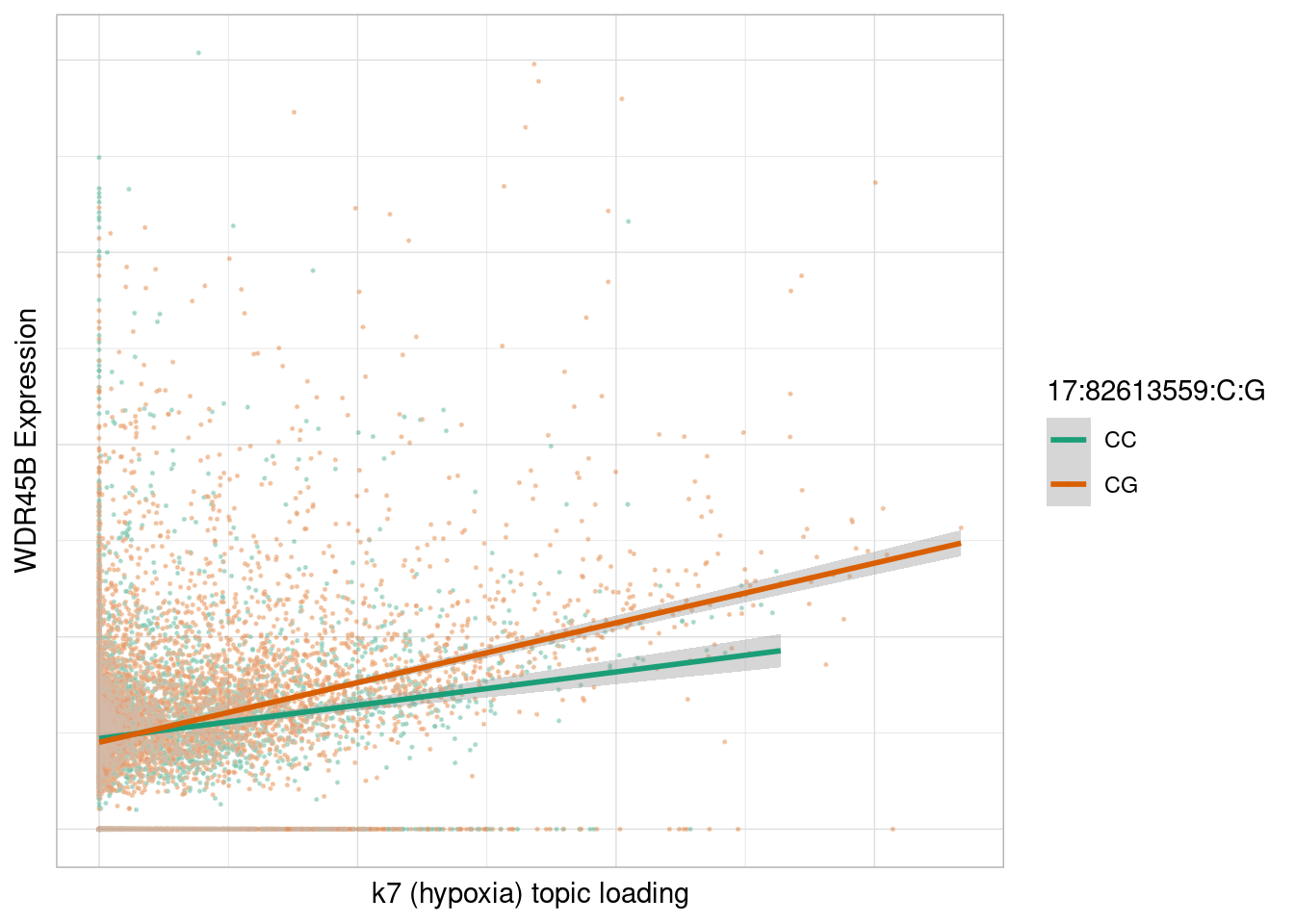

Topic 15. How many of the top correlated eGenes are eGenes in the individual cell types?

beta_topic_corrs_matrix %>% as.data.frame() %>% arrange(desc(abs(k15))) %>% head(n=20) %>% filter(k15>0.6)

                                   k1           k2          k3          k4
RASSF9_12:85870921:G:A    -0.25259654  0.009039522 -0.01394079 -0.08458043
RSPO1_1:37660086:T:C      -0.13148899 -0.051215163  0.09763033 -0.05717446
FOXJ1_17:76100850:G:A     -0.16801281 -0.152483333  0.35623378 -0.22396380
CFAP126_1:161383895:G:C   -0.34071436  0.010831460  0.44134290 -0.28680403
FYB2_1:56825847:A:G       -0.11085152 -0.052060642  0.48209518  0.06543081
SPRY1_4:123365323:C:A     -0.09408339  0.073108477  0.06058185  0.10058601
ABCA1_9:104975539:T:C      0.02363156  0.017305183 -0.03631995  0.04465866
CD44_11:35097776:C:A      -0.03095601 -0.106330539  0.18139729  0.07420194
TMEM132C_12:128218476:C:T -0.13686814 -0.020044243  0.19836120  0.03585012
DYNLRB2_16:80520188:T:C   -0.11683793 -0.078421486  0.30016602 -0.10625551
FN1_2:215434058:T:C       -0.15524752 -0.096517033  0.19126488 -0.03772478
CD151_11:801644:A:T       -0.15803517  0.167638462  0.13729444  0.10256691
                                   k5          k6         k7         k8
RASSF9_12:85870921:G:A     0.11091358  0.02292881 0.08717203 -0.2641889
RSPO1_1:37660086:T:C      -0.09771054 -0.14053840 0.23323145 -0.1434424
FOXJ1_17:76100850:G:A      0.27437715 -0.12591368 0.10315606 -0.1566369
CFAP126_1:161383895:G:C    0.10141447 -0.16103396 0.15964532 -0.2286409
FYB2_1:56825847:A:G        0.12372952  0.25495287 0.22259419 -0.3855926
SPRY1_4:123365323:C:A      0.13458682  0.30278357 0.07450560 -0.4879467
ABCA1_9:104975539:T:C     -0.02363953  0.25729112 0.39194896 -0.4257625
CD44_11:35097776:C:A      -0.11183809  0.37974606 0.52717565 -0.2634827
TMEM132C_12:128218476:C:T -0.25775211 -0.04944711 0.18962611 -0.3037736
DYNLRB2_16:80520188:T:C    0.14606639 -0.18617422 0.02624672 -0.5243134
FN1_2:215434058:T:C       -0.01499032  0.03851312 0.01853084 -0.6084821
CD151_11:801644:A:T        0.03622809  0.26347577 0.21709421 -0.4931014
                                   k9         k10        k11          k12
RASSF9_12:85870921:G:A    -0.28580691 -0.14094440 0.12511856 -0.002659871
RSPO1_1:37660086:T:C      -0.14631804 -0.20890315 0.30815772 -0.099634190
FOXJ1_17:76100850:G:A     -0.11159929 -0.13319220 0.15242846 -0.118279921
CFAP126_1:161383895:G:C   -0.07329987 -0.04050429 0.10409030 -0.056850182
FYB2_1:56825847:A:G       -0.46137549 -0.15089608 0.08068722 -0.197478044
SPRY1_4:123365323:C:A     -0.43538242 -0.07725107 0.22204321  0.043074791
ABCA1_9:104975539:T:C     -0.47641154 -0.19130900 0.18072025 -0.028150674
CD44_11:35097776:C:A      -0.33120002 -0.29568399 0.02221147 -0.409626094
TMEM132C_12:128218476:C:T -0.36162800 -0.23866413 0.47591717  0.080548982
DYNLRB2_16:80520188:T:C   -0.35178526 -0.03300476 0.06580855  0.339363731
FN1_2:215434058:T:C       -0.34705412  0.25951942 0.10343289  0.424049088
CD151_11:801644:A:T       -0.38140939 -0.32031629 0.48018740 -0.097889100
                                  k13         k14       k15
RASSF9_12:85870921:G:A    -0.09255342 -0.15619848 0.9540904
RSPO1_1:37660086:T:C      -0.25444975 -0.15405399 0.9117023
FOXJ1_17:76100850:G:A     -0.11081476 -0.19863064 0.8837666
CFAP126_1:161383895:G:C   -0.18715516 -0.05524329 0.8391898
FYB2_1:56825847:A:G        0.19793486 -0.37950404 0.8066111
SPRY1_4:123365323:C:A     -0.04956571 -0.50351579 0.7971525
ABCA1_9:104975539:T:C      0.09773105 -0.52962342 0.7705794
CD44_11:35097776:C:A       0.38746240 -0.31516744 0.7224227
TMEM132C_12:128218476:C:T -0.01424732 -0.44897227 0.7121441
DYNLRB2_16:80520188:T:C   -0.02755045 -0.35354317 0.7112260
FN1_2:215434058:T:C       -0.24449512 -0.33566665 0.6603629
CD151_11:801644:A:T        0.17928299 -0.53252796 0.6266806

All of these are specific to the cell types associated with topic 15 except CD151, which is also significant in radial glia (of which cortical hem cells are a subset).

g <- "ABCA1"
v <- "9:104975539:T:C"

# pseudocell_exp <- vroom(pseudocell_exp_loc)
genotypes_plink <- read.plink(bed=paste0(plink_prefix, ".bed"),
                        bim=paste0(plink_prefix, ".bim"),
                        fam=paste0(plink_prefix, ".fam"),
                        select.snps = v)
crm_genotypes_df <- tibble("donor"=rownames(genotypes_plink$genotypes), "genotype"=as.numeric(genotypes_plink$genotypes))


pseudocell_df2 <- crm_betas_loadings %>%
  select(all_of(c("PSEUDOCELL", paste0(g, "_", v)))) %>% 
  dplyr::rename(beta_gxc = paste0(g, "_", v)) %>%
  left_join(select(pseudocell_exp, c(pseudocell, eval(g))), by=c("PSEUDOCELL"="pseudocell")) %>%
  mutate(donor=str_extract(PSEUDOCELL, "NA[:digit:]+")) %>% 
  left_join(crm_genotypes_df, by=c("donor")) %>%
  left_join(topic_loadings, by = join_by(PSEUDOCELL==pseudocell)) %>% 
  mutate(genotype=factor(genotype))

ggplot(pseudocell_df2, aes(x=k15, y=ABCA1, color=genotype)) +
  geom_point(size=0.25, alpha = 0.5) * (blend("lighten", alpha = 0.5) + blend("multiply", alpha = 0.1)) +
  geom_smooth(method = "lm") +
  theme_light() +
  scale_color_manual(labels=c("TT", "TC", "CC"), values=brewer.pal(3, "Dark2")) +
  theme(axis.ticks.y=element_blank(), axis.text.y=element_blank(), axis.ticks.x=element_blank(), axis.text.x=element_blank()) +
  xlab("k15 topic loading") +
  ylab("ABCA1 Expression") +
  labs(color=v) 

`geom_smooth()` using formula = 'y ~ x'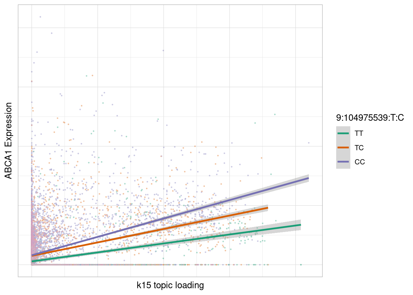

Session information

sessionInfo()

R version 4.2.0 (2022-04-22)
Platform: x86_64-pc-linux-gnu (64-bit)
Running under: CentOS Linux 7 (Core)

Matrix products: default
BLAS/LAPACK: /software/openblas-0.3.13-el7-x86_64/lib/libopenblas_haswellp-r0.3.13.so

locale:
 [1] LC_CTYPE=en_US.UTF-8 LC_NUMERIC=C         LC_TIME=C           
 [4] LC_COLLATE=C         LC_MONETARY=C        LC_MESSAGES=C       
 [7] LC_PAPER=C           LC_NAME=C            LC_ADDRESS=C        
[10] LC_TELEPHONE=C       LC_MEASUREMENT=C     LC_IDENTIFICATION=C 

attached base packages:
[1] stats     graphics  grDevices utils     datasets  methods   base     

other attached packages:
 [1] fastTopics_0.6-142   ggblend_0.1.0        vroom_1.6.4         
 [4] gdata_2.19.0         snpStats_1.46.0      Matrix_1.6-3        
 [7] survival_3.3-1       qvalue_2.28.0        MatrixEQTL_2.3      
[10] ggrepel_0.9.4        udr_0.3-153          mashr_0.2.79        
[13] ashr_2.2-63          viridis_0.6.2        viridisLite_0.4.2   
[16] ggpointdensity_0.1.0 magrittr_2.0.3       pheatmap_1.0.12     
[19] RColorBrewer_1.1-3   pals_1.8             lubridate_1.9.3     
[22] forcats_1.0.0        stringr_1.5.0        dplyr_1.1.4         
[25] purrr_1.0.2          readr_2.1.4          tidyr_1.3.0         
[28] tibble_3.2.1         ggplot2_3.4.4        tidyverse_2.0.0     
[31] SeuratObject_4.1.4   Seurat_4.4.0         workflowr_1.7.0     

loaded via a namespace (and not attached):
  [1] utf8_1.2.4             spatstat.explore_3.0-6 reticulate_1.34.0     
  [4] tidyselect_1.2.0       htmlwidgets_1.6.2      grid_4.2.0            
  [7] Rtsne_0.16             munsell_0.5.0          codetools_0.2-18      
 [10] ica_1.0-3              future_1.33.1          miniUI_0.1.1.1        
 [13] withr_2.5.2            spatstat.random_3.1-3  colorspace_2.1-0      
 [16] progressr_0.14.0       highr_0.9              knitr_1.45            
 [19] rstudioapi_0.17.1      ROCR_1.0-11            tensor_1.5            
 [22] listenv_0.9.1          labeling_0.4.3         git2r_0.30.1          
 [25] mixsqp_0.3-48          polyclip_1.10-0        MCMCpack_1.6-3        
 [28] bit64_4.0.5            farver_2.1.1           rprojroot_2.0.3       
 [31] coda_0.19-4            parallelly_1.37.0      vctrs_0.6.4           
 [34] generics_0.1.3         xfun_0.41              timechange_0.2.0      
 [37] R6_2.5.1               invgamma_1.1           spatstat.utils_3.0-4  
 [40] cachem_1.0.8           assertthat_0.2.1       promises_1.2.0.1      
 [43] scales_1.2.1           gtable_0.3.4           globals_0.16.2        
 [46] processx_3.8.2         goftest_1.2-3          mcmc_0.9-7            
 [49] MatrixModels_0.5-0     rlang_1.1.3            splines_4.2.0         
 [52] lazyeval_0.2.2         dichromat_2.0-0.1      spatstat.geom_3.2-7   
 [55] yaml_2.3.5             reshape2_1.4.4         abind_1.4-5           
 [58] httpuv_1.6.5           tools_4.2.0            ellipsis_0.3.2        
 [61] jquerylib_0.1.4        BiocGenerics_0.44.0    ggridges_0.5.3        
 [64] Rcpp_1.0.12            plyr_1.8.9             progress_1.2.2        
 [67] zlibbioc_1.44.0        prettyunits_1.1.1      ps_1.7.5              
 [70] deldir_1.0-6           pbapply_1.5-0          cowplot_1.1.1         
 [73] zoo_1.8-12             cluster_2.1.3          fs_1.6.3              
 [76] data.table_1.14.8      scattermore_1.2        SparseM_1.81          
 [79] lmtest_0.9-40          RANN_2.6.1             truncnorm_1.0-9       
 [82] mvtnorm_1.2-3          SQUAREM_2021.1         whisker_0.4.1         
 [85] fitdistrplus_1.1-8     matrixStats_1.1.0      hms_1.1.3             
 [88] patchwork_1.1.3        mime_0.12              evaluate_0.23         
 [91] xtable_1.8-4           gridExtra_2.3          compiler_4.2.0        
 [94] maps_3.4.0             KernSmooth_2.23-20     crayon_1.5.2          
 [97] htmltools_0.5.7        mgcv_1.8-40            later_1.3.0           
[100] tzdb_0.4.0             RcppParallel_5.1.5     MASS_7.3-56           
[103] rmeta_3.0              cli_3.6.1              quadprog_1.5-8        
[106] parallel_4.2.0         igraph_1.5.1           pkgconfig_2.0.3       
[109] getPass_0.2-2          sp_2.1-3               plotly_4.10.0         
[112] spatstat.sparse_3.0-3  bslib_0.5.1            callr_3.7.3           
[115] digest_0.6.34          sctransform_0.4.1      RcppAnnoy_0.0.19      
[118] spatstat.data_3.0-3    rmarkdown_2.26         leiden_0.4.2          
[121] uwot_0.1.16            quantreg_5.97          shiny_1.7.5.1         
[124] gtools_3.9.4           lifecycle_1.0.4        nlme_3.1-157          
[127] jsonlite_1.8.7         mapproj_1.2.11         fansi_1.0.5           
[130] pillar_1.9.0           lattice_0.20-45        fastmap_1.1.1         
[133] httr_1.4.7             glue_1.6.2             png_0.1-8             
[136] bit_4.0.5              stringi_1.8.1          sass_0.4.7            
[139] irlba_2.3.5.1          future.apply_1.11.1