figure2

workflowr

• Summary
• Checks
• Past versions

Last updated: 2025-04-19

Checks: 7 0

Knit directory: organoid_oxygen_eqtl/

This reproducible R Markdown analysis was created with workflowr (version 1.7.0). The Checks tab describes the reproducibility checks that were applied when the results were created. The Past versions tab lists the development history.

---

R Markdown file: up-to-date

Great! Since the R Markdown file has been committed to the Git repository, you know the exact version of the code that produced these results.

Environment: empty

Great job! The global environment was empty. Objects defined in the global environment can affect the analysis in your R Markdown file in unknown ways. For reproduciblity it’s best to always run the code in an empty environment.

Seed: set.seed(20250224)

The command set.seed(20250224) was run prior to running the code in the R Markdown file. Setting a seed ensures that any results that rely on randomness, e.g. subsampling or permutations, are reproducible.

Session information: recorded

Great job! Recording the operating system, R version, and package versions is critical for reproducibility.

Cache: none

Nice! There were no cached chunks for this analysis, so you can be confident that you successfully produced the results during this run.

File paths: relative

Great job! Using relative paths to the files within your workflowr project makes it easier to run your code on other machines.

Repository version: 03481ab

Great! You are using Git for version control. Tracking code development and connecting the code version to the results is critical for reproducibility.

The results in this page were generated with repository version 03481ab. See the Past versions tab to see a history of the changes made to the R Markdown and HTML files.

Note that you need to be careful to ensure that all relevant files for the analysis have been committed to Git prior to generating the results (you can use wflow_publish or wflow_git_commit). workflowr only checks the R Markdown file, but you know if there are other scripts or data files that it depends on. Below is the status of the Git repository when the results were generated:

Ignored files:
    Ignored:    .DS_Store
    Ignored:    analysis/.Rhistory
    Ignored:    code/.DS_Store

Unstaged changes:
    Deleted:    code/mash_EE.R
    Modified:   code/mash_EE_PC.R

Note that any generated files, e.g. HTML, png, CSS, etc., are not included in this status report because it is ok for generated content to have uncommitted changes.

---

These are the previous versions of the repository in which changes were made to the R Markdown (analysis/figure2.Rmd) and HTML (docs/figure2.html) files. If you’ve configured a remote Git repository (see ?wflow_git_remote), click on the hyperlinks in the table below to view the files as they were in that past version.

File	Version	Author	Date	Message
Rmd	03481ab	Ben Umans	2025-04-19	updated April 2025
html	9aa3c6e	Ben Umans	2025-02-25	Build site.
Rmd	a6cc51f	Ben Umans	2025-02-25	updated plot formatting
html	e2547f5	Ben Umans	2025-02-24	Build site.
Rmd	1cb030f	Ben Umans	2025-02-24	updated for reviews
Rmd	f0eaf05	Ben Umans	2024-09-05	organized for upload to github
html	f0eaf05	Ben Umans	2024-09-05	organized for upload to github

---

Introduction

This page describes steps used to identify differentially expressed genes from pseudobulk data, classify treatment-responsive cells, plot cell data from immunostained organoid sections, and generate results shown in Figure 2, Figure S2, and Figure S3.

pacman::p_load(edgeR, variancePartition, BiocParallel, limma)
library(Seurat)

Attaching SeuratObject

library(tidyverse)

── Attaching core tidyverse packages ──────────────────────── tidyverse 2.0.0 ──
✔ dplyr     1.1.4     ✔ readr     2.1.4
✔ forcats   1.0.0     ✔ stringr   1.5.0
✔ lubridate 1.9.3     ✔ tibble    3.2.1
✔ purrr     1.0.2     ✔ tidyr     1.3.0

── Conflicts ────────────────────────────────────────── tidyverse_conflicts() ──
✖ dplyr::filter() masks stats::filter()
✖ dplyr::lag()    masks stats::lag()
ℹ Use the conflicted package (<http://conflicted.r-lib.org/>) to force all conflicts to become errors

library(pals)
library(RColorBrewer)
library(ggbreak)

ggbreak v0.1.2

If you use ggbreak in published research, please cite the following
paper:

S Xu, M Chen, T Feng, L Zhan, L Zhou, G Yu. Use ggbreak to effectively
utilize plotting space to deal with large datasets and outliers.
Frontiers in Genetics. 2021, 12:774846. doi: 10.3389/fgene.2021.774846

library(mashr)

Loading required package: ashr

library(udr)
# library(ebnm)
library(pheatmap)
library(ggrepel)
library(knitr)
source("/project/gilad/umans/tools/R_snippets/mash_missing_pieces.R")
source("analysis/shared_functions_style_items.R")

Pseudobulk and DE analysis

Subset data to high quality cells from normoxia, hypoxia, and hyperoxia conditions.

harmony.batchandindividual.sct <- readRDS(file = "/project2/gilad/umans/oxygen_eqtl/output/harmony_organoid_dataset.rds")

subset_seurat <- subset(harmony.batchandindividual.sct, subset = vireo.prob.singlet > 0.95 & nCount_RNA<20000 & nCount_RNA>2500 & treatment != "control21" )

Then, pseudobulk data by individual, collection batch, cell type (coarse or fine), and treatment condition. For comparison, also create pseudobulk dataset that ignores cell type.

pseudo_coarse_quality <- generate.pseudobulk(subset_seurat, labels = c("combined.annotation.coarse.harmony", "treatment", "vireo.individual", "batch"))

pseudo_fine_quality <- generate.pseudobulk(subset_seurat, labels = c("combined.annotation.fine.harmony", "treatment", "vireo.individual", "batch"))

pseudo_all_quality <- generate.pseudobulk(subset_seurat, labels = c("treatment", "batch", "vireo.individual"))

pseudo_fine_quality <- readRDS(file = "/project2/gilad/umans/oxygen_eqtl/output/pseudo_fine_quality_filtered_de_20240305.RDS")
pseudo_coarse_quality <- readRDS(file = "/project2/gilad/umans/oxygen_eqtl/output/pseudo_coarse_quality_filtered_de_20240305.RDS")

We previously determined that filtering to a minimum of 20 cells per pseudobulk sample minimizes excess sample variation associated with cell numbers.

pseudo_coarse_quality_de <- filter.pseudobulk(pseudo_coarse_quality, threshold = 20)
pseudo_fine_quality_de <- filter.pseudobulk(pseudo_fine_quality, threshold = 20)

The following function takes pseudobulk input, splits by a chosen factor (here, cell types), and uses dream to fit a DE model to each group independently.

de_genes_pseudoinput <- function(pseudo_input, classification, model_formula, maineffect, min.count = 5,
                                 min.prop=0.7, min.total.count = 10){
  q <- length(base::unique(pseudo_input$meta[[classification]]))
  pseudo <- vector(mode = "list", length = q)
  names(pseudo) <- unique(pseudo_input$meta[[classification]]) %>% unlist() %>% unname()
  #generate pseudobulk of q+1 clusters
  for (k in names(pseudo)){
    pseudo[[eval(k)]] <- DGEList(pseudo_input$counts[,which(pseudo_input$meta[[classification]]==k)])
    pseudo[[eval(k)]]$samples <- cbind(pseudo[[eval(k)]]$samples[,c("lib.size","norm.factors")], 
                                       pseudo_input$meta[which(pseudo_input$meta[[classification]]==k ),])
    print(k)
  }
  
  print("Partitioned pseudobulk data. Initializing results table.")
  #set up output data structure
  results <- vector(mode = "list", length = q)
  names(results) <- names(pseudo)
  
  print("Results list initialized. Beginning DE testing by cluster.")

#set up DE testing
  for (j in names(pseudo)){
    print(j)
    d <- pseudo[[eval(j)]]
    if(length(base::unique(d$samples[[eval(maineffect)]]))<2){ #prevent testing a cluster that exists in only one condition
      next
    }
    if(length(unique(d$samples[["batch"]]))<2){ #prevent testing a cluster that exists in only one batch; remove if batch is not in the model
      next
    }
    if(length(unique(d$samples[["vireo.individual"]]))<3){ #prevent testing a cluster that exists in only one individual; remove if individual is not in the model
      next
    }
   keepgenes <- filterByExpr(d$counts, group = d$samples[[maineffect]])
    print(paste0("Testing ", sum(keepgenes), " genes"))
    d <- d[keepgenes,]
    d <- calcNormFactors(d, method = "TMM")
    v <- voomWithDreamWeights(d, model_formula, d$samples, plot=FALSE, BPPARAM = param)
    modelfit <- dream(exprObj = v, formula = model_formula, data = d$samples, quiet = TRUE, suppressWarnings = TRUE, BPPARAM = param) #, L = L
 
    print(paste0("Tested cluster ", j, " for DE genes"))
    results[[eval(j)]] <- variancePartition::eBayes(modelfit)

    rm(d, keepgenes, v, modelfit)
    print(paste0("Finished DE testing of cluster ", j))
  }
  return(results)
}

model_formula <- ~  treatment + (1|batch) + (1|vireo.individual) 
param = SnowParam(20, "SOCK", progressbar=TRUE)
bpstopOnError(param) <- FALSE
register(param)

First, obtained results for the coarsely-annotated cell types:

de_results_combinedcoarse_filtered <- de_genes_pseudoinput(pseudo_input = pseudo_coarse_quality_de, classification = "combined.annotation.coarse.harmony", model_formula = model_formula, maineffect = "treatment", min.count = 5, min.prop=0.7, min.total.count = 10)

Because the VLMC cell type exists, after pseudobulk filtering, in only one batch, it wasn’t tested above. I can test it separately:

model_formula_onebatch <- ~  treatment + (1|vireo.individual) 

pseudo_coarse_quality_de_vlmc <- list()
pseudo_coarse_quality_de_vlmc$counts <-  pseudo_coarse_quality_de$counts[,c(which(pseudo_coarse_quality_de$meta$combined.annotation.coarse.harmony=="VLMC"))]
pseudo_coarse_quality_de_vlmc$meta <- pseudo_coarse_quality_de$meta %>% filter(combined.annotation.coarse.harmony == "VLMC")

de_results_combinedcoarse_filtered_vlmc <- de_genes_pseudoinput(pseudo_input = pseudo_coarse_quality_de_vlmc, classification = "combined.annotation.coarse.harmony", model_formula = model_formula_onebatch, maineffect = "treatment", min.count = 5, min.prop=0.7, min.total.count = 10)

de_results_combinedcoarse_filtered[["VLMC"]] <- de_results_combinedcoarse_filtered_vlmc$VLMC

saveRDS(de_results_combinedcoarse_filtered, file = "/project2/gilad/umans/oxygen_eqtl/output/de_results_combinedcoarse_filtered_reharmonize_20240305.RDS")

de_results_combinedcoarse_filtered <- readRDS(file = "/project2/gilad/umans/oxygen_eqtl/output/de_results_combinedcoarse_filtered_reharmonize_20240305.RDS")

Results are given in the supplementary tables:

hypoxia_coarse <- lapply(names(de_results_combinedcoarse_filtered), function(x) topTable(de_results_combinedcoarse_filtered[[x]], coef = "treatmentstim1pct", number = Inf) %>% rownames_to_column(var = "gene"))

hypoxia_coarse_table <- gdata::combine(hypoxia_coarse[[1]], hypoxia_coarse[[2]], hypoxia_coarse[[3]], hypoxia_coarse[[4]], hypoxia_coarse[[5]], hypoxia_coarse[[6]], hypoxia_coarse[[7]], hypoxia_coarse[[8]], hypoxia_coarse[[9]], hypoxia_coarse[[10]], names = names(de_results_combinedcoarse_filtered)) 

write_csv(x = hypoxia_coarse_table, file = "output/hypoxia_de_genes_coarse.csv")

hyperoxia_coarse <- lapply(names(de_results_combinedcoarse_filtered), function(x) topTable(de_results_combinedcoarse_filtered[[x]], coef = "treatmentstim21pct", number = Inf) %>% rownames_to_column(var = "gene"))

hyperoxia_coarse_table <- gdata::combine(hyperoxia_coarse[[1]], hyperoxia_coarse[[2]], hyperoxia_coarse[[3]], hyperoxia_coarse[[4]], hyperoxia_coarse[[5]], hyperoxia_coarse[[6]], hyperoxia_coarse[[7]], hyperoxia_coarse[[8]], hyperoxia_coarse[[9]], hyperoxia_coarse[[10]], names = names(de_results_combinedcoarse_filtered)) 

write_csv(x = hyperoxia_coarse_table, file = "output/hyperoxia_de_genes_coarse.csv")

Now I do the same thing for the fine classification. Oligodendrocytes and midbrain dopaminergic neurons were present in too few individuals for DE analysis after filtering and for simplicity we can censor them up front.

pseudo_fine_quality_de$counts <- pseudo_fine_quality_de$counts[,-c(which(pseudo_fine_quality_de$meta$combined.annotation.fine.harmony=="Oligo"))]
pseudo_fine_quality_de$meta <- pseudo_fine_quality_de$meta %>% filter(combined.annotation.fine.harmony != "Oligo")

pseudo_fine_quality_de$counts <- pseudo_fine_quality_de$counts[,-c(which(pseudo_fine_quality_de$meta$combined.annotation.fine.harmony=="MidbrainDA"))]
pseudo_fine_quality_de$meta <- pseudo_fine_quality_de$meta %>% filter(combined.annotation.fine.harmony != "MidbrainDA")


de_results_combinedfine_filtered <- de_genes_pseudoinput(pseudo_input = pseudo_fine_quality_de, classification = "combined.annotation.fine.harmony", model_formula = model_formula, maineffect = "treatment", min.count = 5, min.prop=0.7, min.total.count = 10)

model_formula_onebatch <- ~  treatment + (1|vireo.individual) 

pseudo_fine_quality_de_vlmc <- list()
pseudo_fine_quality_de_vlmc$counts <-  pseudo_fine_quality_de$counts[,c(which(pseudo_fine_quality_de$meta$combined.annotation.fine.harmony=="VLMC"))]
pseudo_fine_quality_de_vlmc$meta <- pseudo_coarse_quality_de$meta %>% filter(combined.annotation.fine.harmony == "VLMC")

de_results_combinedfine_filtered_vlmc <- de_genes_pseudoinput(pseudo_input = pseudo_fine_quality_de_vlmc, classification = "combined.annotation.fine.harmony", model_formula = model_formula_onebatch, maineffect = "treatment", min.count = 5, min.prop=0.7, min.total.count = 10)

de_results_combinedfine_filtered_vlmc[["VLMC"]] <- de_results_combinedfine_filtered_vlmc$VLMC
saveRDS(de_results_combinedfine_filtered, file = "/project2/gilad/umans/oxygen_eqtl/output/de_results_combinedfine_filtered_reharmonize_20240305.RDS")

de_results_combinedfine_filtered <- readRDS(file = "/project2/gilad/umans/oxygen_eqtl/output/de_results_combinedfine_filtered_reharmonize_20240305.RDS")

Results are given in the supplementary tables:

hypoxia_fine <- lapply(names(de_results_combinedfine_filtered), function(x) topTable(de_results_combinedfine_filtered[[x]], coef = "treatmentstim1pct", number = Inf) %>% rownames_to_column(var = "gene"))
      
hypoxia_fine_table <- gdata::combine(hypoxia_fine[[1]], hypoxia_fine[[2]], hypoxia_fine[[3]], hypoxia_fine[[4]], hypoxia_fine[[5]], hypoxia_fine[[6]], hypoxia_fine[[7]], hypoxia_fine[[8]], hypoxia_fine[[9]], hypoxia_fine[[10]], hypoxia_fine[[11]], hypoxia_fine[[12]], hypoxia_fine[[13]], hypoxia_fine[[14]], hypoxia_fine[[15]], hypoxia_fine[[16]], hypoxia_fine[[17]], hypoxia_fine[[18]], names = names(de_results_combinedfine_filtered)) 

write_csv(x = hypoxia_fine_table, file = "output/hypoxia_de_genes_fine.csv")

hyperoxia_fine <- lapply(names(de_results_combinedfine_filtered), function(x) topTable(de_results_combinedfine_filtered[[x]], coef = "treatmentstim21pct", number = Inf) %>% rownames_to_column(var = "gene"))

hyperoxia_fine_table <- gdata::combine(hyperoxia_fine[[1]], hyperoxia_fine[[2]], hyperoxia_fine[[3]], hyperoxia_fine[[4]], hyperoxia_fine[[5]], hyperoxia_fine[[6]], hyperoxia_fine[[7]], hyperoxia_fine[[8]], hyperoxia_fine[[9]], hyperoxia_fine[[10]], hyperoxia_fine[[11]], hyperoxia_fine[[12]], hyperoxia_fine[[13]], hyperoxia_fine[[14]], hyperoxia_fine[[15]], hyperoxia_fine[[16]], hyperoxia_fine[[17]], hyperoxia_fine[[18]], names = names(de_results_combinedfine_filtered)) 

write_csv(x = hyperoxia_fine_table, file = "output/hyperoxia_de_genes_fine.csv")

Summarize the number of DE genes per cell type, as well as the number of genes tested.

de.summary.fine <-  matrix(0, nrow = length(names(de_results_combinedfine_filtered)), ncol =10)
colnames(de.summary.fine) <-c("hypoxia", "hyperoxia", "ncells_hypoxia", "ncells_hyperoxia", "nindiv_hypoxia", "nindiv_hyperoxia", "hypoxia_mineffect", "hyperoxia_mineffect", "hypoxia_testedgenes", "hyperoxia_testedgenes")
rownames(de.summary.fine) <- names(de_results_combinedfine_filtered)

for (cell in names(de_results_combinedfine_filtered)){
  de.summary.fine[cell, 1] <- sum(topTable(de_results_combinedfine_filtered[[cell]], coef="treatmentstim1pct", number = Inf)$adj.P.Val < 0.05)
  de.summary.fine[cell, 2] <- sum(topTable(de_results_combinedfine_filtered[[cell]], coef="treatmentstim21pct", number = Inf)$adj.P.Val < 0.05)
    de.summary.fine[cell, 3] <- pseudo_fine_quality_de$meta %>% filter(combined.annotation.fine.harmony==cell) %>% dplyr::filter(treatment %in% c("control10", "stim1pct")) %>%  group_by(treatment) %>%  summarize(totals=sum(ncells)) %>% ungroup() %>% summarize(cellnums=mean(totals)) %>% pull(cellnums)
    de.summary.fine[cell, 4] <- pseudo_fine_quality_de$meta %>% filter(combined.annotation.fine.harmony==cell) %>% dplyr::filter(treatment %in% c("control10", "stim21pct")) %>% group_by(treatment) %>%  summarize(totals=sum(ncells)) %>% ungroup() %>% summarize(cellnums=mean(totals)) %>% pull(cellnums)
    de.summary.fine[cell, 5] <- pseudo_fine_quality_de$meta %>% filter(combined.annotation.fine.harmony==cell) %>% dplyr::filter(treatment %in% c("control10", "stim1pct")) %>% pull(vireo.individual) %>% unique() %>% length()
    de.summary.fine[cell, 6] <- pseudo_fine_quality_de$meta %>% filter(combined.annotation.fine.harmony==cell) %>% dplyr::filter(treatment %in% c("control10", "stim21pct")) %>% pull(vireo.individual) %>% unique() %>% length()
    de.summary.fine[cell, 7] <- topTable(de_results_combinedfine_filtered[[cell]], coef="treatmentstim1pct", number = Inf) %>% filter(adj.P.Val < 0.05) %>% filter(abs(logFC)>0.58) %>% nrow() 
  de.summary.fine[cell, 8] <- (topTable(de_results_combinedfine_filtered[[cell]], coef="treatmentstim21pct", number = Inf) %>% filter(adj.P.Val < 0.05) %>% filter(abs(logFC)>0.58) %>% nrow())
  de.summary.fine[cell, 9] <- nrow(topTable(de_results_combinedfine_filtered[[cell]], coef="treatmentstim1pct", number = Inf))
  de.summary.fine[cell, 10] <- nrow(topTable(de_results_combinedfine_filtered[[cell]], coef="treatmentstim21pct", number = Inf))

}

de.summary.fine <- de.summary.fine %>% as.data.frame() %>% arrange(nindiv_hypoxia) %>% rownames_to_column("celltype")

Plot the fraction of tested genes that are DE (to account for the differences in number of tested genes between cell types, which results from different abundances of cell types), along with the fraction that are DE with greater than 1.5-fold change, and the number of tested genes.

ggplot(de.summary.fine, mapping = aes(x=reorder(celltype, hypoxia/hypoxia_testedgenes), y=hypoxia/hypoxia_testedgenes, fill=celltype)) +  geom_bar(stat = "identity", alpha=0.5) + ggtitle("DE summary, fine clusters, hypoxia")  + theme_light() + 
  geom_bar(aes(y=hypoxia_mineffect/hypoxia_testedgenes), stat = "identity", alpha=1) +
  ylab("Fraction of genes differentially expressed") + 
  guides(x =  guide_axis(angle = 45)) + xlab("") + 
  scale_fill_manual(values=manual_palette_fine) + 
  geom_point(aes(x=celltype, y=hypoxia_testedgenes/30000), size=0.8) + 
  geom_line(aes(x=celltype, y=hypoxia_testedgenes/30000, group=1), linewidth=0.3) + 
  theme(legend.position = "none") + 
    scale_y_continuous(name = "Fraction DE Genes", sec.axis = sec_axis(~ . *30000, name="Genes tested"))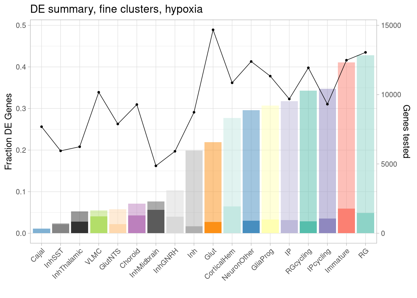 

Past versions of unnamed-chunk-16-1.png

Version	Author	Date
f0eaf05	Ben Umans	2024-09-05

ggplot(de.summary.fine, mapping = aes(x=reorder(celltype, hyperoxia/hyperoxia_testedgenes), y=hyperoxia/hyperoxia_testedgenes, fill=celltype)) +  geom_bar(stat = "identity", alpha=0.5) + ggtitle("DE summary, fine clusters, hyperoxia")  + theme_light() + 
  geom_bar(aes(y=hyperoxia_mineffect/hyperoxia_testedgenes), stat = "identity", alpha=1) +
  ylab("Fraction of genes differentially expressed") + 
  guides(x =  guide_axis(angle = 45)) + xlab("") + 
  scale_fill_manual(values=manual_palette_fine) + 
  geom_point(aes(x=celltype, y=hyperoxia_testedgenes/30000), size=0.8) + 
  geom_line(aes(x=celltype, y=hyperoxia_testedgenes/30000, group=1), linewidth=0.3) + 
  theme(legend.position = "none") + 
    scale_y_continuous(name = "Fraction DE Genes", sec.axis = sec_axis(~ . *30000, name="Genes tested"))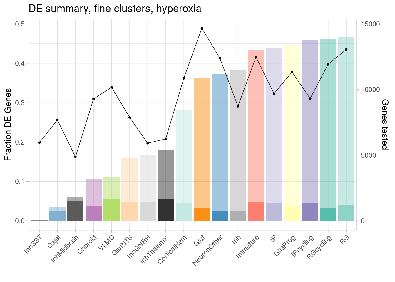 

Past versions of unnamed-chunk-16-2.png

Version	Author	Date
f0eaf05	Ben Umans	2024-09-05

The number of DE genes after hypoxia, aggregated across cell types, is given by:

sapply(c("GlutNTS", "Glut", "NeuronOther" ,"IP" ,"RG", "Inh", "GliaProg", "Immature","CorticalHem", "IPcycling",   "RGcycling", "Choroid",  "Cajal", "InhGNRH", "InhThalamic", "InhMidbrain", "InhSST","VLMC"), function(i) topTable(de_results_combinedfine_filtered[[i]], coef = "treatmentstim1pct", number = Inf, p.value = 0.05) %>% rownames_to_column(var = "gene") %>% pull(gene)) %>% unlist() %>% unname() %>% unique() %>% length()

[1] 10230

Or, restricting to genes with >1.5-fold change:

sapply(c("GlutNTS", "Glut", "NeuronOther" ,"IP" ,"RG", "Inh", "GliaProg", "Immature","CorticalHem", "IPcycling",   "RGcycling", "Choroid",  "Cajal", "InhGNRH", "InhThalamic", "InhMidbrain", "InhSST","VLMC"), function(i) topTable(de_results_combinedfine_filtered[[i]], coef = "treatmentstim1pct", number = Inf, p.value = 0.05) %>% filter(abs(logFC)>0.58) %>% rownames_to_column(var = "gene") %>% pull(gene)) %>% unlist() %>% unname() %>% unique() %>% length()

[1] 2703

And after hyperoxia exposure:

sapply(c("GlutNTS", "Glut", "NeuronOther" ,"IP" ,"RG", "Inh", "GliaProg", "Immature","CorticalHem", "IPcycling",   "RGcycling", "Choroid",  "Cajal", "InhGNRH", "InhThalamic", "InhMidbrain", "InhSST","VLMC"), function(i) topTable(de_results_combinedfine_filtered[[i]], coef = "treatmentstim21pct", number = Inf, p.value = 0.05) %>% rownames_to_column(var = "gene") %>% pull(gene)) %>% unlist() %>% unname() %>% unique() %>% length()

[1] 10425

Or, restricting to genes with >1.5-fold change:

sapply(c("GlutNTS", "Glut", "NeuronOther" ,"IP" ,"RG", "Inh", "GliaProg", "Immature","CorticalHem", "IPcycling",   "RGcycling", "Choroid",  "Cajal", "InhGNRH", "InhThalamic", "InhMidbrain", "InhSST","VLMC"), function(i) topTable(de_results_combinedfine_filtered[[i]], coef = "treatmentstim21pct", number = Inf, p.value = 0.05) %>% filter(abs(logFC)>0.58) %>% rownames_to_column(var = "gene") %>% pull(gene)) %>% unlist() %>% unname() %>% unique() %>% length()

[1] 2855

The same summary for coarsely-clustered cells is similar:

de.summary.coarse <-  matrix(0, nrow = length(names(de_results_combinedcoarse_filtered)), ncol =10)
colnames(de.summary.coarse) <-c("hypoxia", "hyperoxia", "ncells_hypoxia", "ncells_hyperoxia", "nindiv_hypoxia", "nindiv_hyperoxia", "hypoxia_mineffect", "hyperoxia_mineffect", "hypoxia_testedgenes", "hyperoxia_testedgenes")
rownames(de.summary.coarse) <- names(de_results_combinedcoarse_filtered)

# here, I'll count the fraction of tested genes that are DE (hypoxia or hyperoxia) as well as the number of DE genes thresholded to a minimum 1.5-fold change (hypoxia_mineffect or hyperoxia_mineffect).

for (cell in names(de_results_combinedcoarse_filtered)){
  de.summary.coarse[cell, 1] <- sum(topTable(de_results_combinedcoarse_filtered[[cell]], coef="treatmentstim1pct", number = Inf)$adj.P.Val < 0.05)
  de.summary.coarse[cell, 2] <- sum(topTable(de_results_combinedcoarse_filtered[[cell]], coef="treatmentstim21pct", number = Inf)$adj.P.Val < 0.05)
    de.summary.coarse[cell, 3] <- pseudo_coarse_quality_de$meta %>% filter(combined.annotation.coarse.harmony==cell) %>% dplyr::filter(treatment %in% c("control10", "stim1pct")) %>% summarize(total=sum(ncells)) %>% pull(total)
    de.summary.coarse[cell, 4] <- pseudo_coarse_quality_de$meta %>% filter(combined.annotation.coarse.harmony==cell) %>% dplyr::filter(treatment %in% c("control10", "stim21pct")) %>% summarize(total=sum(ncells)) %>% pull(total)
    de.summary.coarse[cell, 5] <- pseudo_coarse_quality_de$meta %>% filter(combined.annotation.coarse.harmony==cell) %>% dplyr::filter(treatment %in% c("control10", "stim1pct")) %>% pull(vireo.individual) %>% unique() %>% length()
    de.summary.coarse[cell, 6] <- pseudo_coarse_quality_de$meta %>% filter(combined.annotation.coarse.harmony==cell) %>% dplyr::filter(treatment %in% c("control10", "stim21pct")) %>% pull(vireo.individual) %>% unique() %>% length()
    de.summary.coarse[cell, 7] <- (topTable(de_results_combinedcoarse_filtered[[cell]], coef="treatmentstim1pct", number = Inf) %>% filter(adj.P.Val < 0.05) %>% filter(abs(logFC)>0.58) %>% nrow() )
  de.summary.coarse[cell, 8] <- (topTable(de_results_combinedcoarse_filtered[[cell]], coef="treatmentstim21pct", number = Inf) %>% filter(adj.P.Val < 0.05) %>% filter(abs(logFC)>0.58) %>% nrow())
  de.summary.coarse[cell, 9] <- topTable(de_results_combinedcoarse_filtered[[cell]], coef="treatmentstim1pct", number = Inf) %>% nrow()
  de.summary.coarse[cell, 10] <- nrow(topTable(de_results_combinedcoarse_filtered[[cell]], coef="treatmentstim21pct", number = Inf))

}

de.summary.coarse <- de.summary.coarse %>% as.data.frame() %>% rownames_to_column("celltype")
de.summary.coarse %>% kable(caption = "DE summary Coarse reharmonized clusters")

DE summary Coarse reharmonized clusters

celltype	hypoxia	hyperoxia	ncells_hypoxia	ncells_hyperoxia	nindiv_hypoxia	nindiv_hyperoxia	hypoxia_mineffect	hyperoxia_mineffect	hypoxia_testedgenes	hyperoxia_testedgenes
Glut	3527	5702	20529	22286	21	20	405	484	15106	15106
NeuronOther	3633	4558	11652	11373	16	19	387	327	12584	12584
IP	4366	5796	9992	11610	20	19	353	460	11553	11553
RG	6761	7896	27763	27422	21	21	598	536	14742	14742
Inh	3302	4798	10749	10993	19	19	304	348	11988	11988
Glia	3275	4837	7188	7933	19	19	406	423	11562	11562
Immature	5221	5408	18376	16927	21	20	757	606	12419	12419
Choroid	468	667	1424	1461	11	11	326	316	8862	8862
Cajal	59	192	665	713	6	6	59	132	7286	7286
VLMC	554	1116	1118	1412	6	7	414	571	10171	10171

Plot the fraction of tested genes that are DE (to account for the differences in number of tested genes between cell types, which results from different abundances of cell types), along with the fraction that are DE with greater than 1.5-fold change, and the number of tested genes.

ggplot(de.summary.coarse, mapping = aes(x=reorder(celltype, hypoxia/hypoxia_testedgenes), y=hypoxia/hypoxia_testedgenes, fill=celltype)) +  geom_bar(stat = "identity", alpha=0.5) + ggtitle("DE summary, fine clusters, hypoxia")  + theme_light() + 
  geom_bar(aes(y=hypoxia_mineffect/hypoxia_testedgenes), stat = "identity", alpha=1) +
  ylab("Fraction of genes differentially expressed") + 
  guides(x =  guide_axis(angle = 45)) + xlab("") + 
  scale_fill_manual(values=manual_palette_fine) + 
  geom_point(aes(x=celltype, y=hypoxia_testedgenes/30000), size=0.8) + 
  geom_line(aes(x=celltype, y=hypoxia_testedgenes/30000, group=1), linewidth=0.3) + 
  theme(legend.position = "none") + 
    scale_y_continuous(name = "Fraction DE Genes", sec.axis = sec_axis(~ . *30000, name="Genes tested"))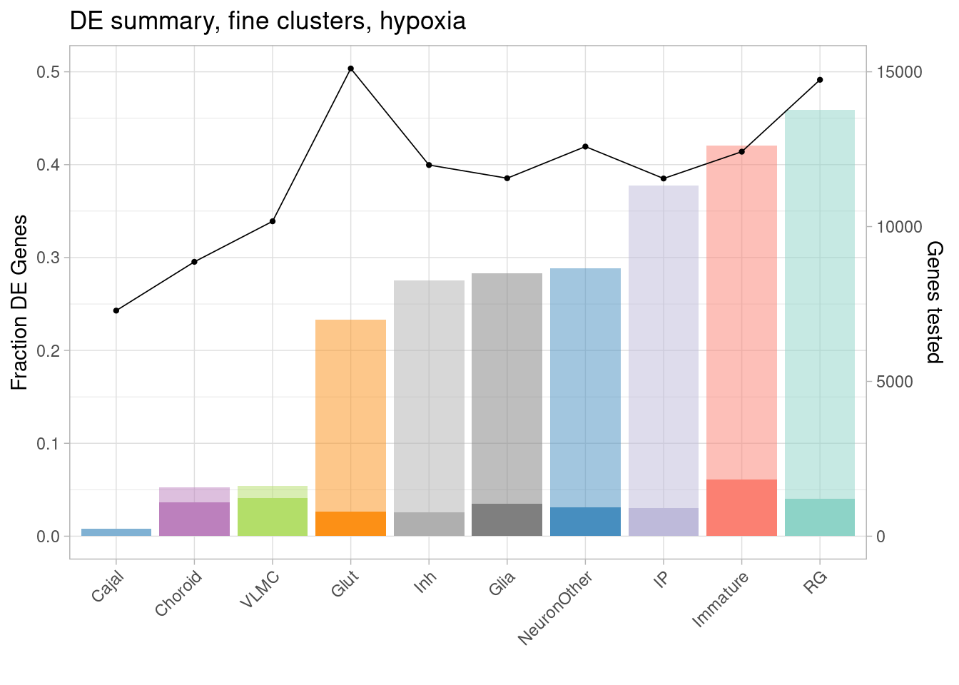 

Past versions of unnamed-chunk-22-1.png

Version	Author	Date
e2547f5	Ben Umans	2025-02-24
f0eaf05	Ben Umans	2024-09-05

ggplot(de.summary.coarse, mapping = aes(x=reorder(celltype, hyperoxia/hyperoxia_testedgenes), y=hyperoxia/hyperoxia_testedgenes, fill=celltype)) +  geom_bar(stat = "identity", alpha=0.5) + ggtitle("DE summary, fine clusters, hyperoxia")  + theme_light() + 
  geom_bar(aes(y=hyperoxia_mineffect/hyperoxia_testedgenes), stat = "identity", alpha=1) +
  ylab("Fraction of genes differentially expressed") + 
  guides(x =  guide_axis(angle = 45)) + xlab("") + 
  scale_fill_manual(values=manual_palette_fine) + 
  geom_point(aes(x=celltype, y=hyperoxia_testedgenes/30000), size=0.8) + 
  geom_line(aes(x=celltype, y=hyperoxia_testedgenes/30000, group=1), linewidth=0.3) + 
  theme(legend.position = "none") + 
    scale_y_continuous(name = "Fraction DE Genes", sec.axis = sec_axis(~ . *30000, name="Genes tested"))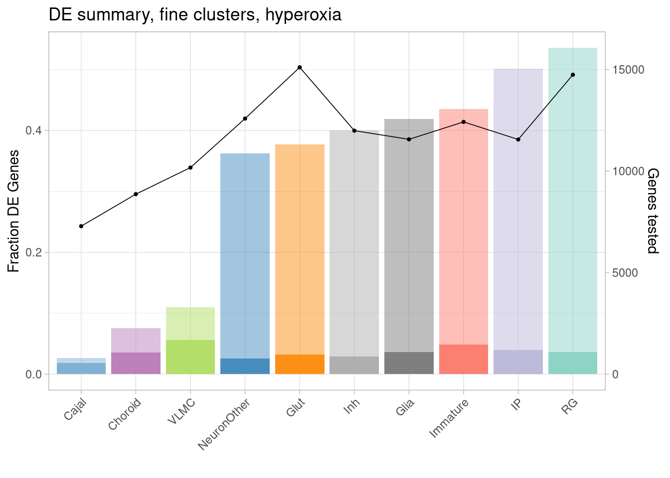 

Past versions of unnamed-chunk-22-2.png

Version	Author	Date
e2547f5	Ben Umans	2025-02-24
f0eaf05	Ben Umans	2024-09-05

The number of hypoxia DE genes aggregated across cell types is given by:

sapply(c("Glut", "NeuronOther" ,"IP" ,"RG", "Inh", "Glia", "Immature", "Choroid",  "Cajal", "VLMC"), function(i) topTable(de_results_combinedcoarse_filtered[[i]], coef = "treatmentstim1pct", number = Inf, p.value = 0.05)  %>% rownames_to_column(var = "gene") %>% pull(gene)) %>% unlist() %>% unname() %>% unique() %>% length()

[1] 10466

Or, restricting to >1.5-fold change:

sapply(c("Glut", "NeuronOther" ,"IP" ,"RG", "Inh", "Glia", "Immature", "Choroid",  "Cajal", "VLMC"), function(i) topTable(de_results_combinedcoarse_filtered[[i]], coef = "treatmentstim1pct", number = Inf, p.value = 0.05) %>% filter(abs(logFC)>0.58) %>% rownames_to_column(var = "gene") %>% pull(gene)) %>% unlist() %>% unname() %>% unique() %>% length()

[1] 2068

For hyperoxia, this is given by: The number of hypoxia DE genes aggregated across cell types is given by:

sapply(c("Glut", "NeuronOther" ,"IP" ,"RG", "Inh", "Glia", "Immature", "Choroid",  "Cajal", "VLMC"), function(i) topTable(de_results_combinedcoarse_filtered[[i]], coef = "treatmentstim21pct", number = Inf, p.value = 0.05)  %>% rownames_to_column(var = "gene") %>% pull(gene)) %>% unlist() %>% unname() %>% unique() %>% length()

[1] 10754

Or, restricting to >1.5-fold change:

sapply(c("Glut", "NeuronOther" ,"IP" ,"RG", "Inh", "Glia", "Immature", "Choroid",  "Cajal", "VLMC"), function(i) topTable(de_results_combinedcoarse_filtered[[i]], coef = "treatmentstim21pct", number = Inf, p.value = 0.05) %>% filter(abs(logFC)>0.58) %>% rownames_to_column(var = "gene") %>% pull(gene)) %>% unlist() %>% unname() %>% unique() %>% length()

[1] 2053

Ignoring cell type information yields a different number of DE genes:

results_all <- readRDS(file = "/project2/gilad/umans/oxygen_eqtl/output/de_results_pseudoall_filtered_20231107.RDS")

sum(topTable(results_all, coef="treatmentstim1pct", number = Inf)$adj.P.Val < 0.05)

[1] 8611

sum(topTable(results_all, coef="treatmentstim21pct", number = Inf)$adj.P.Val < 0.05)

[1] 10509

If we restrict this to genes with >1.5fold change in expression:

topTable(results_all, coef="treatmentstim1pct", number = Inf) %>% filter(adj.P.Val < 0.05) %>% filter(abs(logFC)>0.58) %>% nrow()

[1] 815

topTable(results_all, coef="treatmentstim21pct", number = Inf) %>% filter(adj.P.Val < 0.05) %>% filter(abs(logFC)>0.58) %>% nrow()

[1] 948

There is a relationship between the number of DE genes and the number of cells (or, equivalently, individuals) tested, but that’s not a complete explanation. Instead, it seems to have a larger impact for detecting small effect sizes:

ggplot(de.summary.fine, mapping = aes(x=ncells_hypoxia, y=hypoxia, label=celltype)) + 
  geom_point(aes(size=nindiv_hypoxia, color=celltype)) + 
  geom_text_repel() + 
  ggtitle("DE summary fine clusters, hypoxia") +  
  # geom_smooth(method = "lm", se = FALSE, color="black", lty=2) + 
  theme_light() +
  scale_color_manual(values=manual_palette_fine) +
  theme(legend.position="none") + scale_x_log10() +
  xlab("Number of cells in comparison") +
  ylab("Number of DE genes")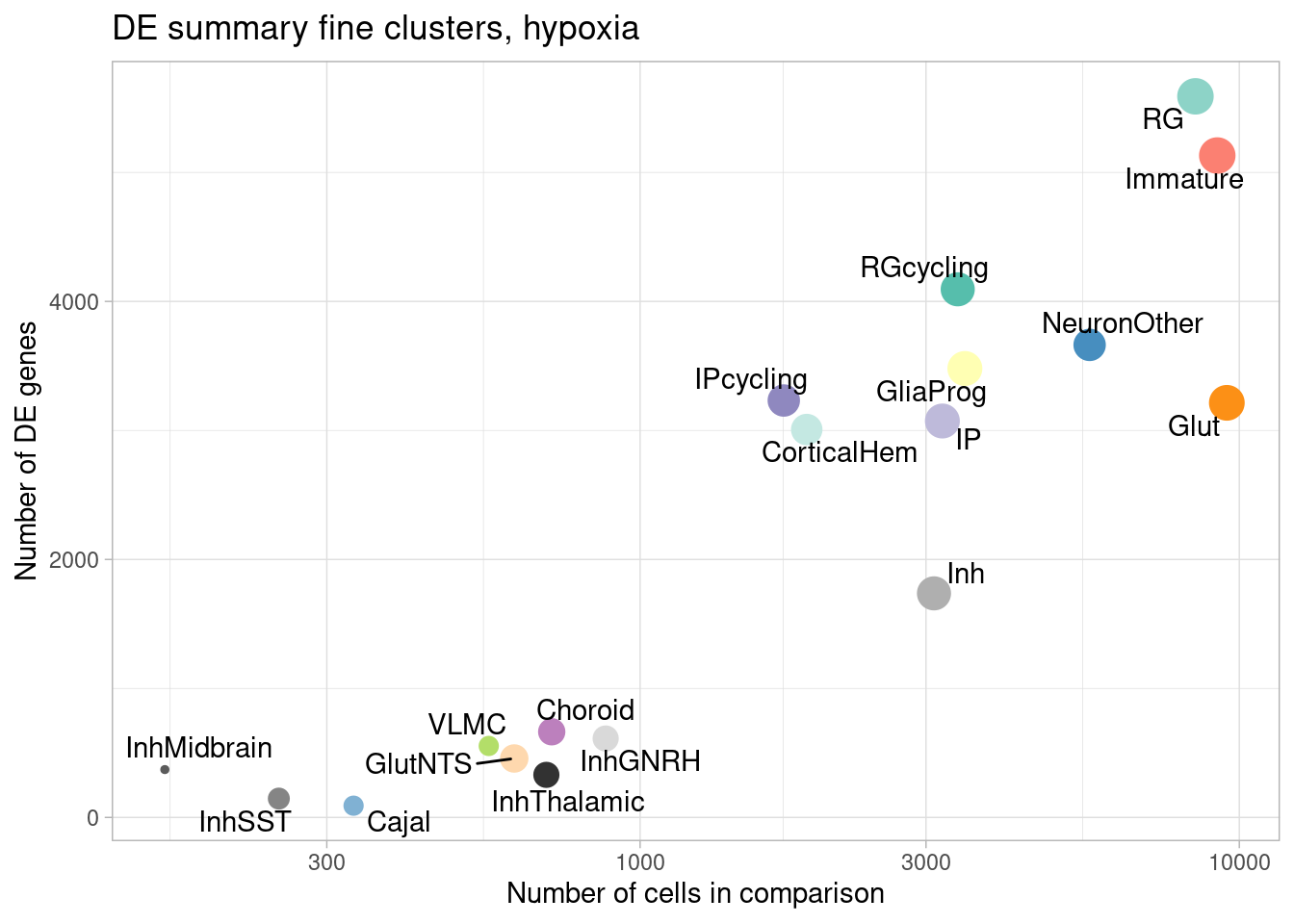

Past versions of unnamed-chunk-29-1.png

Version	Author	Date
f0eaf05	Ben Umans	2024-09-05

ggplot(de.summary.fine, mapping = aes(x=nindiv_hypoxia, y=hypoxia, label=celltype)) + 
  geom_point(aes(size=nindiv_hypoxia, color=celltype)) + 
  geom_text_repel() + 
  ggtitle("DE summary fine clusters, hypoxia") +  
  # geom_smooth(method = "lm", se = FALSE, color="black", lty=2) + 
  theme_light() +
  scale_color_manual(values=manual_palette_fine) +
  theme(legend.position="none") + 
  xlab("Number of individuals in comparison") +
  ylab("Number of DE genes")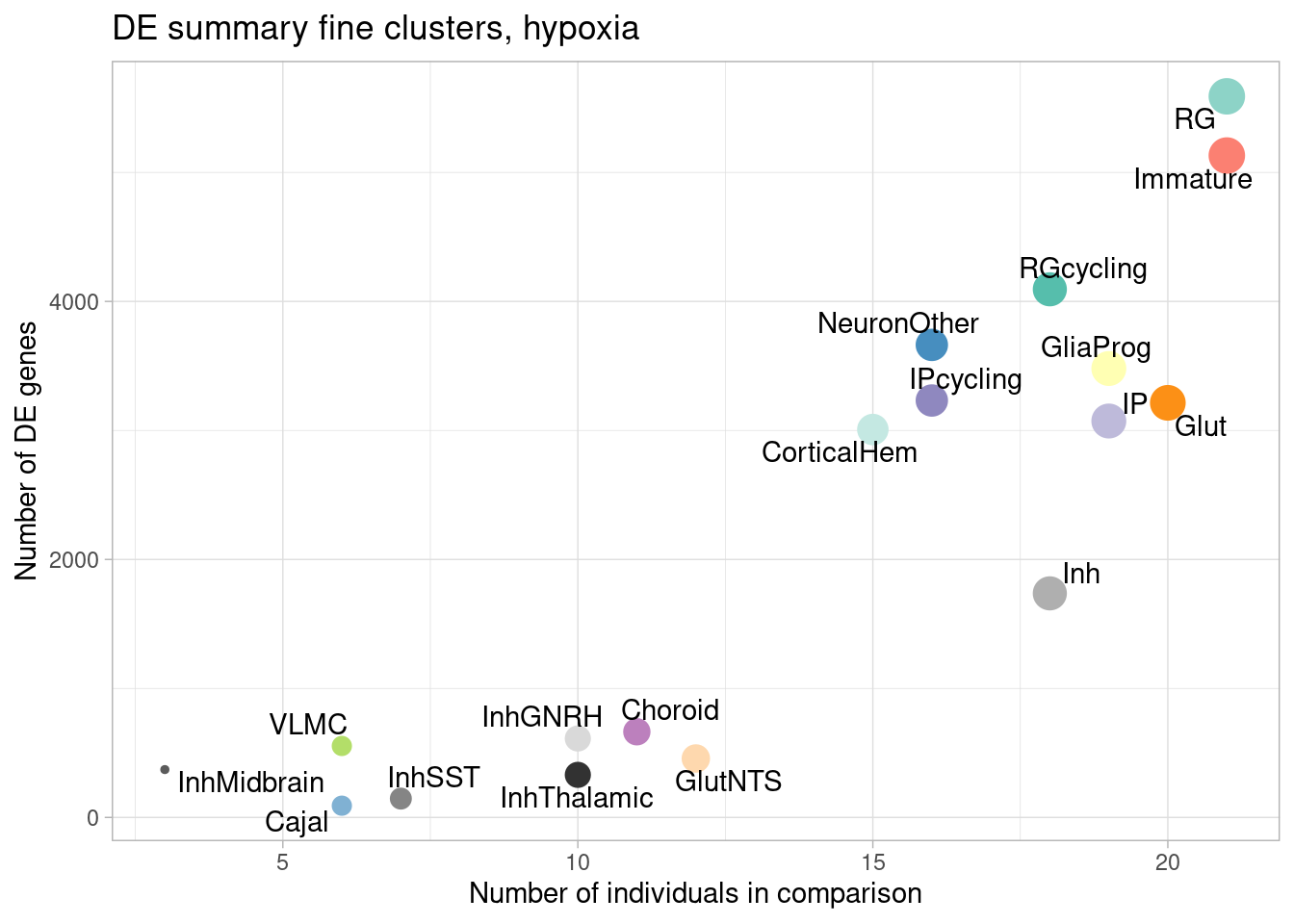

Past versions of unnamed-chunk-29-2.png

Version	Author	Date
f0eaf05	Ben Umans	2024-09-05

ggplot(de.summary.fine, mapping = aes(x=nindiv_hypoxia, y=hypoxia/hypoxia_testedgenes, label=celltype)) + 
  geom_point(aes(size=nindiv_hypoxia, color=celltype)) + 
  geom_text_repel() + 
  ggtitle("DE summary fine clusters, hypoxia") +  
  # geom_smooth(method = "lm", se = FALSE, color="black", lty=2) + 
  theme_light() +
  scale_color_manual(values=manual_palette_fine) +
  theme(legend.position="none") + 
  xlab("Number of individuals in comparison") +
  ylab("Fraction of genes DE")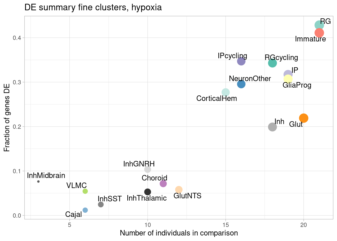

Past versions of unnamed-chunk-29-3.png

Version	Author	Date
f0eaf05	Ben Umans	2024-09-05

ggplot(de.summary.fine, mapping = aes(x=nindiv_hypoxia, y=hypoxia_mineffect, label=celltype)) + 
  geom_point(aes(size=nindiv_hypoxia, color=celltype)) + 
  geom_text_repel() + 
  ggtitle("DE summary fine clusters, hypoxia, >1.5fold effect size") +  
  # geom_smooth(method = "lm", se = FALSE, color="black", lty=2, lwd=0.5) + 
  theme_light() +
  scale_color_manual(values=manual_palette_fine) +
  theme(legend.position="none") + 
  xlab("Number of individuals in comparison") +
  ylab("Number of DE genes")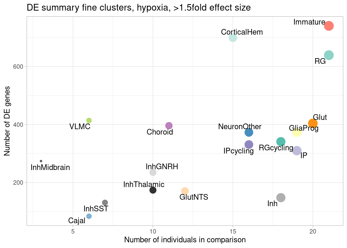

Past versions of unnamed-chunk-29-4.png

Version	Author	Date
f0eaf05	Ben Umans	2024-09-05

ggplot(de.summary.fine, mapping = aes(x=nindiv_hypoxia, y=hypoxia_mineffect/hypoxia_testedgenes, label=celltype)) + 
  geom_point(aes(size=nindiv_hypoxia, color=celltype)) + 
  geom_text_repel() + 
  ggtitle("DE summary fine clusters, hypoxia, >1.5fold effect size") +  
  # geom_smooth(method = "lm", se = FALSE, color="black", lty=2, lwd=0.5) + 
  theme_light() +
  scale_color_manual(values=manual_palette_fine) +
  theme(legend.position="none") + 
  xlab("Number of individuals in comparison") +
  ylab("Fraction of genes DE")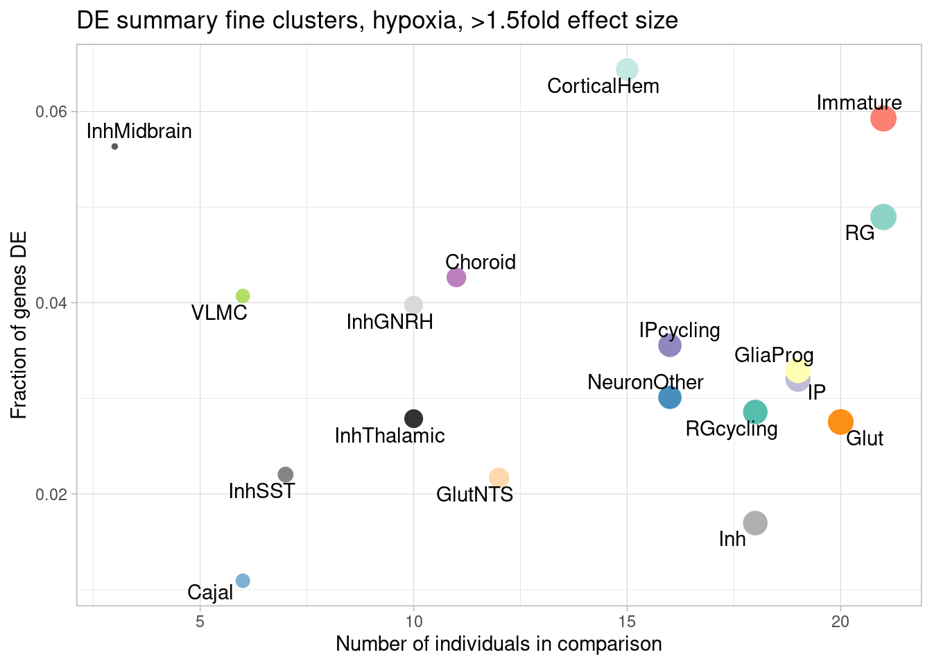

Past versions of unnamed-chunk-29-5.png

Version	Author	Date
f0eaf05	Ben Umans	2024-09-05

Number of individuals, rather than number of cells per pseudobulk sample, is the important factor contributing to power here. We separately found that including cell numbers as a covariation in the DE model has no effect on the relationship shown above, nor do differences in transcriptome size between cell types (constraining all comparisons to a common transcriptome preserved this relationship).

We can look at a variance partition plot (from dream package) to get an approximate sense of the relative contribution of cell type identity, cell line, treatment, and collection batch to overall data variation. We expect that cell type makes the largest contribution here.

vardata <- DGEList(counts = pseudo_fine_quality_de$counts, samples = pseudo_fine_quality_de$meta)
keepgenes <- filterByExpr(y = vardata, min.count = 5, 
                           min.prop=0.4, 
                           min.total.count = 10)

print(paste0("Testing ", sum(keepgenes), " genes"))
vardata <- vardata[keepgenes,]
vardata <- calcNormFactors(vardata, method = "TMM")

formula_all <- ~ (1|combined.annotation.fine.harmony) +  (1|treatment) + (1|vireo.individual) + (1|batch) 
voomed.varpart.all <- voomWithDreamWeights(vardata, formula_all, vardata$samples, plot=TRUE, BPPARAM = param)

vp <- fitExtractVarPartModel(voomed.varpart.all, formula_all, vardata$samples, BPPARAM = param)
saveRDS(vp, "/project2/gilad/umans/oxygen_eqtl/output/vp.RDS")

vp <- readRDS("/project2/gilad/umans/oxygen_eqtl/output/vp.RDS")
plotVarPart(sortCols(vp), size=0.1)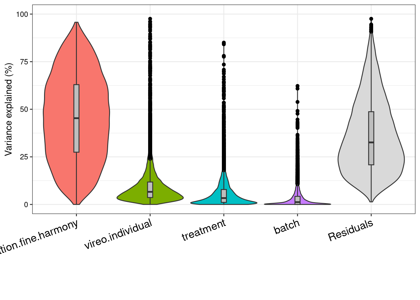

Past versions of unnamed-chunk-31-1.png

Version	Author	Date
e2547f5	Ben Umans	2025-02-24

mash for DE results

Because of differential power between cell types, we run the risk of underestimating how many DE effects are shared between different cell types or conditions. Here, I use mash to estimate posterior effect sizes and significance metrics.

library(mashr)
library(udr)
library(flashier)

## Function to estimate residual covariance for udr
estimate_null_cov_simple = function(data, z_thresh=2, est_cor = TRUE){
  z = data$Bhat/data$Shat
  max_absz = apply(abs(z),1, max)
  nullish = which(max_absz < z_thresh)
  # the null-z vs. number of conditions.
  if(length(nullish)<ncol(z)){
    stop("not enough null data to estimate null correlation")
  }
  nullish_Bhat= data$Bhat[nullish,]
  Vhat = cov(nullish_Bhat)
  if(est_cor){
    Vhat = cov2cor(Vhat)
  }
  return(Vhat)
}

First, repeat the DE above, omitting variancePartition::eBayes(modelfit), as this shrinkage will be done by mash.

de_genes_pseudoinput_for_mash <- function(pseudo_input, classification, model_formula, maineffect, min.count = 5,
                                 min.prop=0.7, min.total.count = 10){
  q <- length(base::unique(pseudo_input$meta[[classification]]))
  pseudo <- vector(mode = "list", length = q)
  names(pseudo) <- unique(pseudo_input$meta[[classification]]) %>% unlist() %>% unname()
  #generate pseudobulk of q+1 clusters
  for (k in names(pseudo)){
    pseudo[[eval(k)]] <- DGEList(pseudo_input$counts[,which(pseudo_input$meta[[classification]]==k)])
    pseudo[[eval(k)]]$samples <- cbind(pseudo[[eval(k)]]$samples[,c("lib.size","norm.factors")], 
                                       pseudo_input$meta[which(pseudo_input$meta[[classification]]==k ),])
    print(k)
  }
  
  print("Partitioned pseudobulk data. Initializing results table.")
  #set up output data structure
  results <- vector(mode = "list", length = q)
  names(results) <- names(pseudo)
  
  print("Results list initialized. Beginning DE testing by cluster.")

#set up DE testing
  for (j in names(pseudo)){
    print(j)
    d <- pseudo[[eval(j)]]
    if(length(base::unique(d$samples[[eval(maineffect)]]))<2){ #prevent testing a cluster that exists in only one condition
      next
    }
    if(length(unique(d$samples[["batch"]]))<2){ #prevent testing a cluster that exists in only one batch; remove if batch is not in the model
      next
    }
    if(length(unique(d$samples[["vireo.individual"]]))<3){ #prevent testing a cluster that exists in only one individual; remove if individual is not in the model
      next
    }
   keepgenes <- filterByExpr(d$counts, group = d$samples[[maineffect]])
    print(paste0("Testing ", sum(keepgenes), " genes"))
    d <- d[keepgenes,]
    d <- calcNormFactors(d, method = "TMM")
    v <- voomWithDreamWeights(d, model_formula, d$samples, plot=FALSE, BPPARAM = param)
    modelfit <- dream(exprObj = v, formula = model_formula, data = d$samples, quiet = TRUE, suppressWarnings = TRUE, BPPARAM = param) #, L = L
 
    print(paste0("Tested cluster ", j, " for DE genes"))
    results[[eval(j)]] <- modelfit

    rm(d, keepgenes, v, modelfit)
    print(paste0("Finished DE testing of cluster ", j))
  }
  return(results)
}

model_formula <- ~  treatment + (1|batch) + (1|vireo.individual) 
param = SnowParam(20, "SOCK", progressbar=TRUE)
bpstopOnError(param) <- FALSE
register(param)

pseudo_fine_quality_de$counts <- pseudo_fine_quality_de$counts[,-c(which(pseudo_fine_quality_de$meta$combined.annotation.fine.harmony=="Oligo"))]
pseudo_fine_quality_de$meta <- pseudo_fine_quality_de$meta %>% filter(combined.annotation.fine.harmony != "Oligo")

pseudo_fine_quality_de$counts <- pseudo_fine_quality_de$counts[,-c(which(pseudo_fine_quality_de$meta$combined.annotation.fine.harmony=="MidbrainDA"))]
pseudo_fine_quality_de$meta <- pseudo_fine_quality_de$meta %>% filter(combined.annotation.fine.harmony != "MidbrainDA")

de_results_combinedfine_filtered_mash <- de_genes_pseudoinput_for_mash(pseudo_input = pseudo_fine_quality_de, classification = "combined.annotation.fine.harmony", model_formula = model_formula, maineffect = "treatment", min.count = 5, min.prop=0.7, min.total.count = 10)

model_formula_onebatch <- ~  treatment + (1|vireo.individual) 

pseudo_fine_quality_de_vlmc <- list()
pseudo_fine_quality_de_vlmc$counts <-  pseudo_fine_quality_de$counts[,c(which(pseudo_fine_quality_de$meta$combined.annotation.fine.harmony=="VLMC"))]
pseudo_fine_quality_de_vlmc$meta <- pseudo_fine_quality_de$meta %>% filter(combined.annotation.fine.harmony == "VLMC")

de_results_combinedfine_filtered_vlmc <- de_genes_pseudoinput_for_mash(pseudo_input = pseudo_fine_quality_de_vlmc, classification = "combined.annotation.fine.harmony", model_formula = model_formula_onebatch, maineffect = "treatment", min.count = 5, min.prop=0.7, min.total.count = 10)

de_results_combinedfine_filtered_mash[["VLMC"]] <- de_results_combinedfine_filtered_vlmc$VLMC

saveRDS(de_results_combinedfine_filtered_mash, file =  "/project2/gilad/umans/oxygen_eqtl/output/de_results_combinedfine_filtered_reharmonize_for_mash_20240731.RDS")

res <- topTable(de_results_combinedfine_filtered_mash[["Glut"]], coef = "treatmentstim1pct", number = Inf) %>% rownames_to_column(var = "gene") %>%  dplyr::select(gene, Glut1=logFC) 

res <- topTable(de_results_combinedfine_filtered_mash[["RG"]], coef = "treatmentstim1pct", number = Inf) %>% rownames_to_column(var = "gene") %>%  dplyr::select(gene, RG1=logFC) %>% full_join(res)

res <- topTable(de_results_combinedfine_filtered_mash[["IP"]], coef = "treatmentstim1pct", number = Inf) %>% rownames_to_column(var = "gene") %>%  dplyr::select(gene, IP1=logFC) %>% full_join(res)

res <- topTable(de_results_combinedfine_filtered_mash[["Immature"]], coef = "treatmentstim1pct", number = Inf) %>% rownames_to_column(var = "gene") %>%  dplyr::select(gene, Immature1=logFC) %>% full_join(res)

res <- topTable(de_results_combinedfine_filtered_mash[["NeuronOther"]], coef = "treatmentstim1pct", number = Inf) %>% rownames_to_column(var = "gene") %>%  dplyr::select(gene, NeuronOther1=logFC) %>% full_join(res)

res <- topTable(de_results_combinedfine_filtered_mash[["VLMC"]], coef = "treatmentstim1pct", number = Inf) %>% rownames_to_column(var = "gene") %>%  dplyr::select(gene, VLMC1=logFC) %>% full_join(res)

res <- topTable(de_results_combinedfine_filtered_mash[["Choroid"]], coef = "treatmentstim1pct", number = Inf) %>% rownames_to_column(var = "gene") %>%  dplyr::select(gene, Choroid1=logFC) %>% full_join(res)

res <- topTable(de_results_combinedfine_filtered_mash[["Cajal"]], coef = "treatmentstim1pct", number = Inf) %>% rownames_to_column(var = "gene") %>%  dplyr::select(gene, Cajal1=logFC) %>% full_join(res)

res <- topTable(de_results_combinedfine_filtered_mash[["Inh"]], coef = "treatmentstim1pct", number = Inf) %>% rownames_to_column(var = "gene") %>%  dplyr::select(gene, Inh1=logFC) %>% full_join(res)

##
res <- topTable(de_results_combinedfine_filtered_mash[["CorticalHem"]], coef = "treatmentstim1pct", number = Inf) %>% rownames_to_column(var = "gene") %>%  dplyr::select(gene, CorticalHem1=logFC) %>% full_join(res)
res <- topTable(de_results_combinedfine_filtered_mash[["GliaProg"]], coef = "treatmentstim1pct", number = Inf) %>% rownames_to_column(var = "gene") %>%  dplyr::select(gene, GliaProg1=logFC) %>% full_join(res)
res <- topTable(de_results_combinedfine_filtered_mash[["GlutNTS"]], coef = "treatmentstim1pct", number = Inf) %>% rownames_to_column(var = "gene") %>%  dplyr::select(gene, GlutNTS1=logFC) %>% full_join(res)
res <- topTable(de_results_combinedfine_filtered_mash[["IPcycling"]], coef = "treatmentstim1pct", number = Inf) %>% rownames_to_column(var = "gene") %>%  dplyr::select(gene, IPcycling1=logFC) %>% full_join(res)
res <- topTable(de_results_combinedfine_filtered_mash[["InhGNRH"]], coef = "treatmentstim1pct", number = Inf) %>% rownames_to_column(var = "gene") %>%  dplyr::select(gene, InhGNRH1=logFC) %>% full_join(res)
res <- topTable(de_results_combinedfine_filtered_mash[["InhMidbrain"]], coef = "treatmentstim1pct", number = Inf) %>% rownames_to_column(var = "gene") %>%  dplyr::select(gene, InhMidbrain1=logFC) %>% full_join(res)
res <- topTable(de_results_combinedfine_filtered_mash[["InhSST"]], coef = "treatmentstim1pct", number = Inf) %>% rownames_to_column(var = "gene") %>%  dplyr::select(gene, InhSST1=logFC) %>% full_join(res)
res <- topTable(de_results_combinedfine_filtered_mash[["InhThalamic"]], coef = "treatmentstim1pct", number = Inf) %>% rownames_to_column(var = "gene") %>%  dplyr::select(gene, InhThalamic1=logFC) %>% full_join(res)
res <- topTable(de_results_combinedfine_filtered_mash[["RGcycling"]], coef = "treatmentstim1pct", number = Inf) %>% rownames_to_column(var = "gene") %>%  dplyr::select(gene, RGcycling1=logFC) %>% full_join(res)

##
res <- topTable(de_results_combinedfine_filtered_mash[["Glut"]], coef = "treatmentstim21pct", number = Inf) %>% rownames_to_column(var = "gene") %>%  dplyr::select(gene, Glut21=logFC) %>% full_join(res)

res <- topTable(de_results_combinedfine_filtered_mash[["RG"]], coef = "treatmentstim21pct", number = Inf) %>% rownames_to_column(var = "gene") %>%  dplyr::select(gene, RG21=logFC) %>% full_join(res)

res <- topTable(de_results_combinedfine_filtered_mash[["IP"]], coef = "treatmentstim21pct", number = Inf) %>% rownames_to_column(var = "gene") %>%  dplyr::select(gene, IP21=logFC) %>% full_join(res)
res <- topTable(de_results_combinedfine_filtered_mash[["Immature"]], coef = "treatmentstim21pct", number = Inf) %>% rownames_to_column(var = "gene") %>%  dplyr::select(gene, Immature21=logFC) %>% full_join(res)
res <- topTable(de_results_combinedfine_filtered_mash[["NeuronOther"]], coef = "treatmentstim21pct", number = Inf) %>% rownames_to_column(var = "gene") %>%  dplyr::select(gene, NeuronOther21=logFC) %>% full_join(res)

res <- topTable(de_results_combinedfine_filtered_mash[["VLMC"]], coef = "treatmentstim21pct", number = Inf) %>% rownames_to_column(var = "gene") %>%  dplyr::select(gene, VLMC21=logFC) %>% full_join(res)

res <- topTable(de_results_combinedfine_filtered_mash[["Choroid"]], coef = "treatmentstim21pct", number = Inf) %>% rownames_to_column(var = "gene") %>%  dplyr::select(gene, Choroid21=logFC) %>% full_join(res)

res <- topTable(de_results_combinedfine_filtered_mash[["Cajal"]], coef = "treatmentstim21pct", number = Inf) %>% rownames_to_column(var = "gene") %>%  dplyr::select(gene, Cajal21=logFC) %>% full_join(res)

res <- topTable(de_results_combinedfine_filtered_mash[["Inh"]], coef = "treatmentstim21pct", number = Inf) %>% rownames_to_column(var = "gene") %>%  dplyr::select(gene, Inh21=logFC) %>% full_join(res)
##
res <- topTable(de_results_combinedfine_filtered_mash[["CorticalHem"]], coef = "treatmentstim21pct", number = Inf) %>% rownames_to_column(var = "gene") %>%  dplyr::select(gene, CorticalHem21=logFC) %>% full_join(res)
res <- topTable(de_results_combinedfine_filtered_mash[["GliaProg"]], coef = "treatmentstim21pct", number = Inf) %>% rownames_to_column(var = "gene") %>%  dplyr::select(gene, GliaProg21=logFC) %>% full_join(res)
res <- topTable(de_results_combinedfine_filtered_mash[["GlutNTS"]], coef = "treatmentstim21pct", number = Inf) %>% rownames_to_column(var = "gene") %>%  dplyr::select(gene, GlutNTS21=logFC) %>% full_join(res)
res <- topTable(de_results_combinedfine_filtered_mash[["IPcycling"]], coef = "treatmentstim21pct", number = Inf) %>% rownames_to_column(var = "gene") %>%  dplyr::select(gene, IPcycling21=logFC) %>% full_join(res)
res <- topTable(de_results_combinedfine_filtered_mash[["InhGNRH"]], coef = "treatmentstim21pct", number = Inf) %>% rownames_to_column(var = "gene") %>%  dplyr::select(gene, InhGNRH21=logFC) %>% full_join(res)
res <- topTable(de_results_combinedfine_filtered_mash[["InhMidbrain"]], coef = "treatmentstim21pct", number = Inf) %>% rownames_to_column(var = "gene") %>%  dplyr::select(gene, InhMidbrain21=logFC) %>% full_join(res)
res <- topTable(de_results_combinedfine_filtered_mash[["InhSST"]], coef = "treatmentstim21pct", number = Inf) %>% rownames_to_column(var = "gene") %>%  dplyr::select(gene, InhSST21=logFC) %>% full_join(res)
res <- topTable(de_results_combinedfine_filtered_mash[["InhThalamic"]], coef = "treatmentstim21pct", number = Inf) %>% rownames_to_column(var = "gene") %>%  dplyr::select(gene, InhThalamic21=logFC) %>% full_join(res)
res <- topTable(de_results_combinedfine_filtered_mash[["RGcycling"]], coef = "treatmentstim21pct", number = Inf) %>% rownames_to_column(var = "gene") %>%  dplyr::select(gene, RGcycling21=logFC) %>% full_join(res)

mash_de_effect <- res %>%  `rownames<-` (.$gene) %>% dplyr::select(-gene)

# And the standard errors

se <- topTable(de_results_combinedfine_filtered_mash[["Glut"]], coef = "treatmentstim1pct", number = Inf) %>% rownames_to_column(var = "gene") %>% mutate(Glut1=logFC/t) %>%  dplyr::select(gene, Glut1) 

se <- topTable(de_results_combinedfine_filtered_mash[["RG"]], coef = "treatmentstim1pct", number = Inf) %>% rownames_to_column(var = "gene") %>% mutate(RG1=logFC/t) %>%  dplyr::select(gene, RG1) %>% full_join(se)

se <- topTable(de_results_combinedfine_filtered_mash[["IP"]], coef = "treatmentstim1pct", number = Inf) %>% rownames_to_column(var = "gene") %>% mutate(IP1=logFC/t) %>%  dplyr::select(gene, IP1) %>% full_join(se)
se <- topTable(de_results_combinedfine_filtered_mash[["Immature"]], coef = "treatmentstim1pct", number = Inf) %>% rownames_to_column(var = "gene") %>% mutate(Immature1=logFC/t) %>%  dplyr::select(gene, Immature1) %>% full_join(se)
se <- topTable(de_results_combinedfine_filtered_mash[["NeuronOther"]], coef = "treatmentstim1pct", number = Inf) %>% rownames_to_column(var = "gene") %>% mutate(NeuronOther1=logFC/t) %>%   dplyr::select(gene, NeuronOther1) %>% full_join(se)

se <- topTable(de_results_combinedfine_filtered_mash[["VLMC"]], coef = "treatmentstim1pct", number = Inf) %>% rownames_to_column(var = "gene") %>% mutate(VLMC1=logFC/t) %>%  dplyr::select(gene, VLMC1) %>% full_join(se)

se <- topTable(de_results_combinedfine_filtered_mash[["Choroid"]], coef = "treatmentstim1pct", number = Inf) %>% rownames_to_column(var = "gene") %>% mutate(Choroid1=logFC/t) %>%  dplyr::select(gene, Choroid1) %>% full_join(se)

se <- topTable(de_results_combinedfine_filtered_mash[["Cajal"]], coef = "treatmentstim1pct", number = Inf) %>% rownames_to_column(var = "gene") %>% mutate(Cajal1=logFC/t) %>%  dplyr::select(gene, Cajal1) %>% full_join(se)
se <- topTable(de_results_combinedfine_filtered_mash[["Inh"]], coef = "treatmentstim1pct", number = Inf) %>% rownames_to_column(var = "gene") %>% mutate(Inh1=logFC/t) %>%  dplyr::select(gene, Inh1) %>% full_join(se)
##
se <- topTable(de_results_combinedfine_filtered_mash[["CorticalHem"]], coef = "treatmentstim1pct", number = Inf) %>% rownames_to_column(var = "gene") %>%  mutate(CorticalHem1=logFC/t) %>%  dplyr::select(gene, CorticalHem1) %>% full_join(se)
se <- topTable(de_results_combinedfine_filtered_mash[["GliaProg"]], coef = "treatmentstim1pct", number = Inf) %>% rownames_to_column(var = "gene")%>% mutate(GliaProg1=logFC/t) %>%  dplyr::select(gene, GliaProg1) %>% full_join(se)
se <- topTable(de_results_combinedfine_filtered_mash[["GlutNTS"]], coef = "treatmentstim1pct", number = Inf) %>% rownames_to_column(var = "gene") %>% mutate(GlutNTS1=logFC/t) %>%  dplyr::select(gene, GlutNTS1) %>% full_join(se)
se <- topTable(de_results_combinedfine_filtered_mash[["IPcycling"]], coef = "treatmentstim1pct", number = Inf) %>% rownames_to_column(var = "gene") %>% mutate(IPcycling1=logFC/t) %>%  dplyr::select(gene, IPcycling1) %>% full_join(se)
se <- topTable(de_results_combinedfine_filtered_mash[["InhGNRH"]], coef = "treatmentstim1pct", number = Inf) %>% rownames_to_column(var = "gene") %>% mutate(InhGNRH1=logFC/t) %>%  dplyr::select(gene, InhGNRH1) %>% full_join(se)
se <- topTable(de_results_combinedfine_filtered_mash[["InhMidbrain"]], coef = "treatmentstim1pct", number = Inf) %>% rownames_to_column(var = "gene") %>% mutate(InhMidbrain1=logFC/t) %>%  dplyr::select(gene, InhMidbrain1) %>% full_join(se)
se <- topTable(de_results_combinedfine_filtered_mash[["InhSST"]], coef = "treatmentstim1pct", number = Inf) %>% rownames_to_column(var = "gene") %>% mutate(InhSST1=logFC/t) %>%  dplyr::select(gene, InhSST1) %>% full_join(se)
se <- topTable(de_results_combinedfine_filtered_mash[["InhThalamic"]], coef = "treatmentstim1pct", number = Inf) %>% rownames_to_column(var = "gene") %>% mutate(InhThalamic1=logFC/t) %>%  dplyr::select(gene, InhThalamic1) %>% full_join(se)
se <- topTable(de_results_combinedfine_filtered_mash[["RGcycling"]], coef = "treatmentstim1pct", number = Inf) %>% rownames_to_column(var = "gene") %>% mutate(RGcycling1=logFC/t) %>%  dplyr::select(gene, RGcycling1) %>% full_join(se)


se <- topTable(de_results_combinedfine_filtered_mash[["Glut"]], coef = "treatmentstim21pct", number = Inf) %>% rownames_to_column(var = "gene") %>% mutate(Glut21=logFC/t) %>%  dplyr::select(gene, Glut21) %>% full_join(se)

se <- topTable(de_results_combinedfine_filtered_mash[["RG"]], coef = "treatmentstim21pct", number = Inf) %>% rownames_to_column(var = "gene") %>% mutate(RG21=logFC/t) %>%  dplyr::select(gene, RG21) %>% full_join(se)

se <- topTable(de_results_combinedfine_filtered_mash[["IP"]], coef = "treatmentstim21pct", number = Inf) %>% rownames_to_column(var = "gene") %>% mutate(IP21=logFC/t) %>%  dplyr::select(gene, IP21) %>% full_join(se)
se <- topTable(de_results_combinedfine_filtered_mash[["Immature"]], coef = "treatmentstim21pct", number = Inf) %>% rownames_to_column(var = "gene") %>% mutate(Immature21=logFC/t) %>%  dplyr::select(gene, Immature21) %>% full_join(se)
se <- topTable(de_results_combinedfine_filtered_mash[["NeuronOther"]], coef = "treatmentstim21pct", number = Inf) %>% rownames_to_column(var = "gene") %>% mutate(NeuronOther21=logFC/t) %>%   dplyr::select(gene, NeuronOther21) %>% full_join(se)

se <- topTable(de_results_combinedfine_filtered_mash[["VLMC"]], coef = "treatmentstim21pct", number = Inf) %>% rownames_to_column(var = "gene") %>% mutate(VLMC21=logFC/t) %>%  dplyr::select(gene, VLMC21) %>% full_join(se)

se <- topTable(de_results_combinedfine_filtered_mash[["Choroid"]], coef = "treatmentstim21pct", number = Inf) %>% rownames_to_column(var = "gene") %>% mutate(Choroid21=logFC/t) %>%  dplyr::select(gene, Choroid21) %>% full_join(se)

se <- topTable(de_results_combinedfine_filtered_mash[["Cajal"]], coef = "treatmentstim21pct", number = Inf) %>% rownames_to_column(var = "gene") %>% mutate(Cajal21=logFC/t) %>%  dplyr::select(gene, Cajal21) %>% full_join(se)
se <- topTable(de_results_combinedfine_filtered_mash[["Inh"]], coef = "treatmentstim21pct", number = Inf) %>% rownames_to_column(var = "gene") %>% mutate(Inh21=logFC/t) %>%  dplyr::select(gene, Inh21) %>% full_join(se)
##
se <- topTable(de_results_combinedfine_filtered_mash[["CorticalHem"]], coef = "treatmentstim21pct", number = Inf) %>% rownames_to_column(var = "gene") %>%  mutate(CorticalHem21=logFC/t) %>%  dplyr::select(gene, CorticalHem21) %>% full_join(se)
se <- topTable(de_results_combinedfine_filtered_mash[["GliaProg"]], coef = "treatmentstim21pct", number = Inf) %>% rownames_to_column(var = "gene")%>% mutate(GliaProg21=logFC/t) %>%  dplyr::select(gene, GliaProg21) %>% full_join(se)
se <- topTable(de_results_combinedfine_filtered_mash[["GlutNTS"]], coef = "treatmentstim21pct", number = Inf) %>% rownames_to_column(var = "gene") %>% mutate(GlutNTS21=logFC/t) %>%  dplyr::select(gene, GlutNTS21) %>% full_join(se)
se <- topTable(de_results_combinedfine_filtered_mash[["IPcycling"]], coef = "treatmentstim21pct", number = Inf) %>% rownames_to_column(var = "gene") %>% mutate(IPcycling21=logFC/t) %>%  dplyr::select(gene, IPcycling21) %>% full_join(se)
se <- topTable(de_results_combinedfine_filtered_mash[["InhGNRH"]], coef = "treatmentstim21pct", number = Inf) %>% rownames_to_column(var = "gene") %>% mutate(InhGNRH21=logFC/t) %>%  dplyr::select(gene, InhGNRH21) %>% full_join(se)
se <- topTable(de_results_combinedfine_filtered_mash[["InhMidbrain"]], coef = "treatmentstim21pct", number = Inf) %>% rownames_to_column(var = "gene") %>% mutate(InhMidbrain21=logFC/t) %>%  dplyr::select(gene, InhMidbrain21) %>% full_join(se)
se <- topTable(de_results_combinedfine_filtered_mash[["InhSST"]], coef = "treatmentstim21pct", number = Inf) %>% rownames_to_column(var = "gene") %>% mutate(InhSST21=logFC/t) %>%  dplyr::select(gene, InhSST21) %>% full_join(se)
se <- topTable(de_results_combinedfine_filtered_mash[["InhThalamic"]], coef = "treatmentstim21pct", number = Inf) %>% rownames_to_column(var = "gene") %>% mutate(InhThalamic21=logFC/t) %>%  dplyr::select(gene, InhThalamic21) %>% full_join(se)
se <- topTable(de_results_combinedfine_filtered_mash[["RGcycling"]], coef = "treatmentstim21pct", number = Inf) %>% rownames_to_column(var = "gene") %>% mutate(RGcycling21=logFC/t) %>%  dplyr::select(gene, RGcycling21) %>% full_join(se)
##

mash_de_se <- se %>%  `rownames<-` (.$gene) %>% dplyr::select(-gene)

mash_dataset9 <- mash_set_data(as.matrix(mash_de_effect), as.matrix(mash_de_se), alpha = 1)
#set up cov matrix
##select strong signals
m.1by1 <- mash_1by1(mash_dataset9)
strong <- get_significant_results(m.1by1, 0.01)

#account for correlations
V.simple = estimate_null_correlation_simple(mash_dataset9, z_thresh = 3)
data.Vsimple = mash_update_data(mash_dataset9, V=V.simple)

dat.strong = list(data.Vsimple$Bhat[strong, ], data.Vsimple$Shat[strong, ])
names(dat.strong) = c("Bhat", "Shat")
dat.random = list(data.Vsimple$Bhat[-strong, ], data.Vsimple$Shat[-strong, ])
names(dat.random) = c("Bhat", "Shat")

#cannonical covariance using all the tests
U.c = cov_canonical(data.Vsimple) 
#data-driven covariance using flashr + pca
U.f = cov_flash(data.Vsimple, subset = strong)
U.pca = cov_pca(data.Vsimple,ifelse(ncol(mash_de_effect)<5, ncol(mash_de_effect), 5),subset=strong)

# Denoised data-driven matrices
# Initialization of udr 
maxiter=1e3
U.init = c(U.f, U.pca)
Vhat = estimate_null_cov_simple(dat.random, est_cor = FALSE)
fit0 <- ud_init(dat.strong$Bhat, U_scaled = U.c, n_rank1 = 0, U_unconstrained = U.init, V = Vhat)

# fit udr model
fit1 <- ud_fit(fit0, control = list(unconstrained.update = "ted", maxiter = maxiter, tol = 1e-2, tol.lik = 1e-2))

# extract data-driven covariance from udr model. (A list of covariance matrices)
U.ted <- lapply(fit1$U,function (e) "[["(e,"mat"))

#fit mash model to all the tests
m.Vsimple = mash(data.Vsimple, c(U.c, U.ted)) 
#compute posterior stat
m_posterior <- mash_compute_posterior_matrices(m.Vsimple, data.Vsimple)
saveRDS(m.Vsimple, file="output/mash_de/mashmodel_dataset9_fine_reharmonized_z3.RDS")
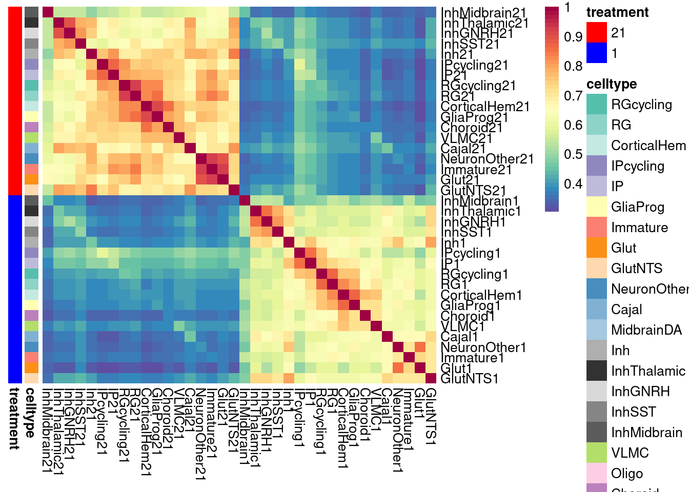
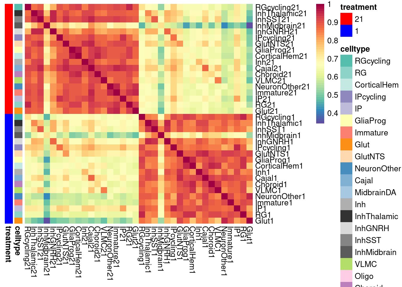
saveRDS(m_posterior, file="output/mash_de/mashposterior_dataset9_fine_reharmonized_z3.RDS")

Using these posterior results, I define “shared” effects between any two conditions as those that are (a) significant in at least one of the conditions and (b) differ in magnitude by less than a factor of 2.5, with the same sign.

The matrix of sharing by these criteria is obtained from:

m_posterior <- readRDS(file="/project2/gilad/umans/oxygen_eqtl/output/mash_de/mashposterior_dataset9_fine_reharmonized_z3.RDS")

shared.size = matrix(NA,nrow = ncol(m_posterior$lfsr),ncol=ncol(m_posterior$lfsr))
colnames(shared.size) <- rownames(shared.size) <-colnames(m_posterior$lfsr)
for (i in 1:ncol(m_posterior$lfsr)) {
  for (j in 1:ncol(m_posterior$lfsr)) {
    sig.row=which(m_posterior$lfsr[,i] < 0.05)
    sig.col=which(m_posterior$lfsr[,j] < 0.05)
    a=(union(sig.row,sig.col)) # at least one effect is significant
    quotient=(m_posterior$PosteriorMean[a,i]/m_posterior$PosteriorMean[a,j])
    shared.size[i,j] = mean(quotient > 0.4 & quotient < 2.5)
  }
}

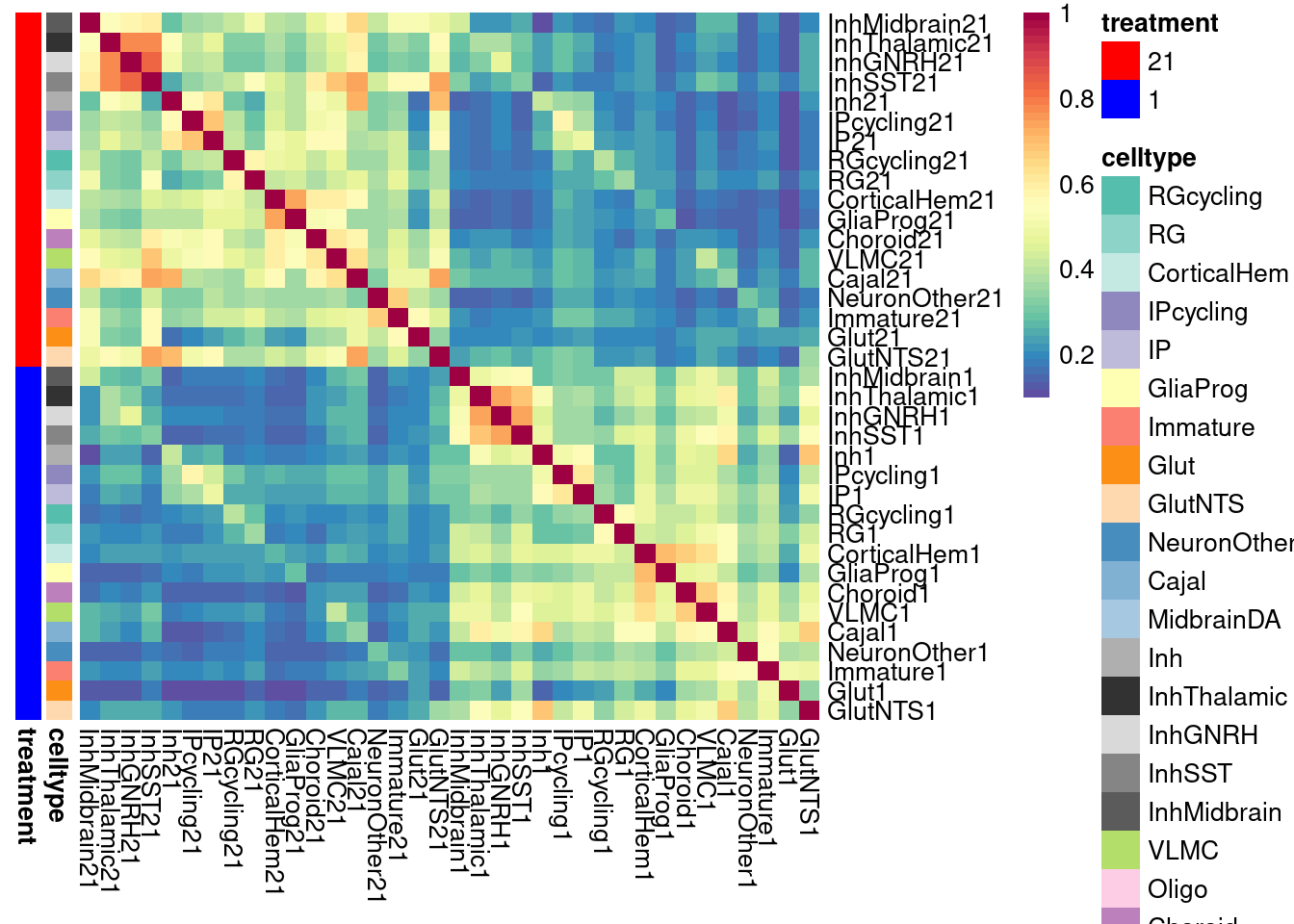
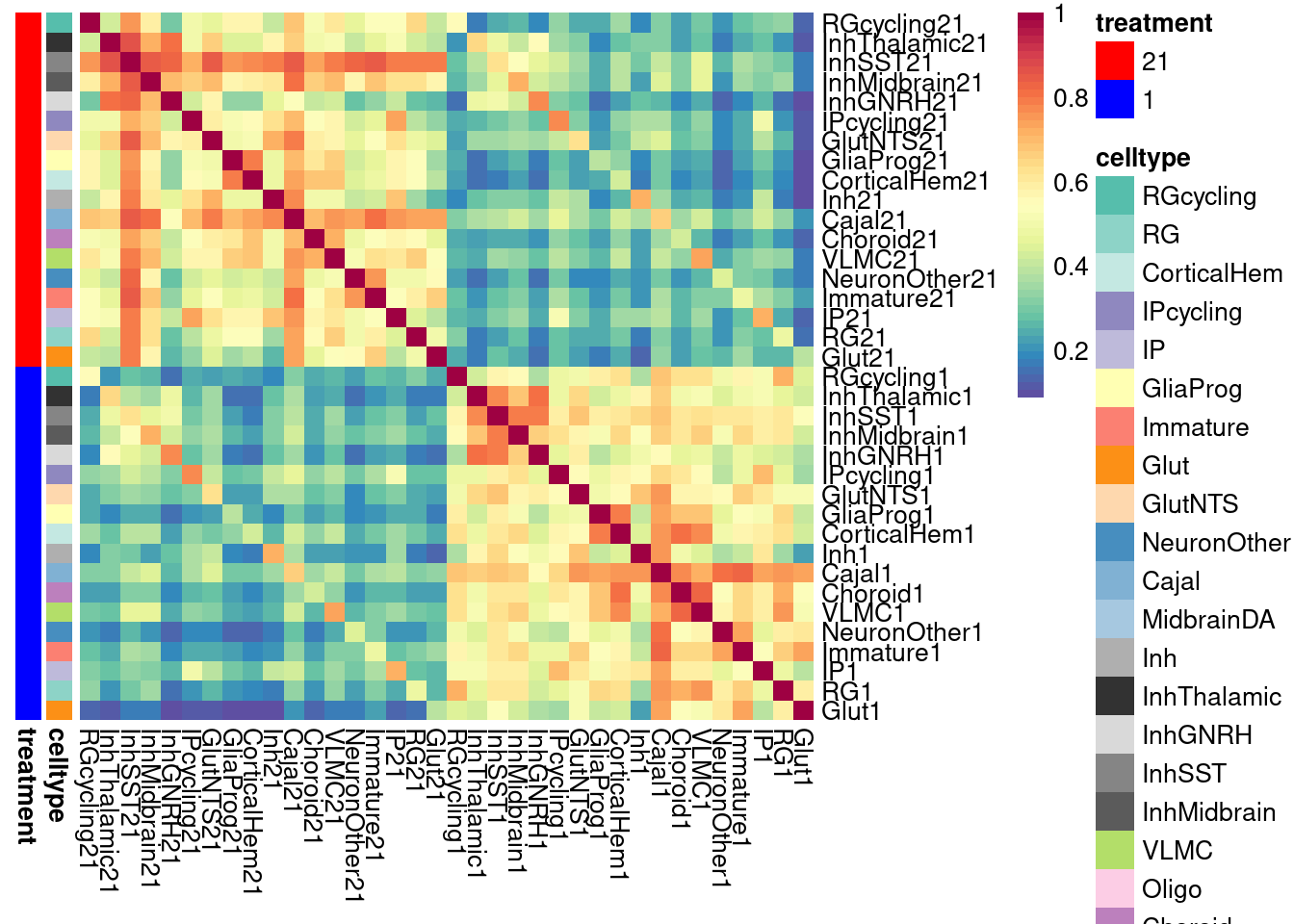
# alternatively, additionally constrain to a minimum logFC
shared.size.constrained = matrix(NA,nrow = ncol(m_posterior$lfsr),ncol=ncol(m_posterior$lfsr))
colnames(shared.size.constrained) <- rownames(shared.size.constrained) <-colnames(m_posterior$lfsr)
for (i in 1:ncol(m_posterior$lfsr)) {
  for (j in 1:ncol(m_posterior$lfsr)) {
    sig.row=which(m_posterior$lfsr[,i] < 0.05)
    sig.col=which(m_posterior$lfsr[,j] < 0.05)
    size.row=which(abs(m_posterior$PosteriorMean[,i]) > 0.58)
    size.col=which(abs(m_posterior$PosteriorMean[,j]) > 0.58)
    a=intersect(union(sig.row,sig.col), union(size.row, size.col)) # at least one effect is significant
    # constrain to those with at least one posterior mean logFC>0.58
    quotient=(m_posterior$PosteriorMean[a,i]/m_posterior$PosteriorMean[a,j])
    shared.size.constrained[i,j] = mean(quotient > 0.4 & quotient < 2.5 )
  }
}


# reorder the rows and columns for consistent display

shared.size <- shared.size[c( "InhMidbrain21", "InhThalamic21", "InhGNRH21", "InhSST21",   "Inh21", "IPcycling21", "IP21",  "RGcycling21", "RG21",  "CorticalHem21", "GliaProg21",   "Choroid21", "VLMC21",  "Cajal21", "NeuronOther21", "Immature21", "Glut21", "GlutNTS21", "InhMidbrain1", "InhThalamic1", "InhGNRH1", "InhSST1",   "Inh1",  "IPcycling1", "IP1",  "RGcycling1", "RG1",  "CorticalHem1", "GliaProg1",  "Choroid1", "VLMC1", "Cajal1",  "NeuronOther1",  "Immature1", "Glut1", "GlutNTS1"),  
                          c( "InhMidbrain21", "InhThalamic21", "InhGNRH21", "InhSST21",   "Inh21", "IPcycling21", "IP21",  "RGcycling21", "RG21",  "CorticalHem21", "GliaProg21",   "Choroid21", "VLMC21",  "Cajal21", "NeuronOther21", "Immature21", "Glut21", "GlutNTS21", "InhMidbrain1", "InhThalamic1", "InhGNRH1", "InhSST1",   "Inh1",  "IPcycling1", "IP1",  "RGcycling1", "RG1",  "CorticalHem1", "GliaProg1",  "Choroid1", "VLMC1", "Cajal1",  "NeuronOther1",  "Immature1", "Glut1", "GlutNTS1")]

shared.size.constrained <- shared.size.constrained[c( "InhMidbrain21", "InhThalamic21", "InhGNRH21", "InhSST21",   "Inh21", "IPcycling21", "IP21",  "RGcycling21", "RG21",  "CorticalHem21", "GliaProg21",   "Choroid21", "VLMC21",  "Cajal21", "NeuronOther21", "Immature21", "Glut21", "GlutNTS21", "InhMidbrain1", "InhThalamic1", "InhGNRH1", "InhSST1",   "Inh1",  "IPcycling1", "IP1",  "RGcycling1", "RG1",  "CorticalHem1", "GliaProg1",  "Choroid1", "VLMC1", "Cajal1",  "NeuronOther1",  "Immature1", "Glut1", "GlutNTS1"),  
                          c( "InhMidbrain21", "InhThalamic21", "InhGNRH21", "InhSST21",   "Inh21", "IPcycling21", "IP21",  "RGcycling21", "RG21",  "CorticalHem21", "GliaProg21",   "Choroid21", "VLMC21",  "Cajal21", "NeuronOther21", "Immature21", "Glut21", "GlutNTS21", "InhMidbrain1", "InhThalamic1", "InhGNRH1", "InhSST1",   "Inh1",  "IPcycling1", "IP1",  "RGcycling1", "RG1",  "CorticalHem1", "GliaProg1",  "Choroid1", "VLMC1", "Cajal1",  "NeuronOther1",  "Immature1", "Glut1", "GlutNTS1")]



# intersection instead of union
shared.size.intersection = matrix(NA,nrow = ncol(m_posterior$lfsr),ncol=ncol(m_posterior$lfsr))
colnames(shared.size.intersection) <- rownames(shared.size.intersection) <-colnames(m_posterior$lfsr)
for (i in 1:ncol(m_posterior$lfsr)) {
  for (j in 1:ncol(m_posterior$lfsr)) {
    sig.row=which(m_posterior$lfsr[,i] < 0.05)
    sig.col=which(m_posterior$lfsr[,j] < 0.05)
    a=(intersect(sig.row,sig.col)) # at least one effect is significant
    quotient=(m_posterior$PosteriorMean[a,i]/m_posterior$PosteriorMean[a,j])
    shared.size.intersection[i,j] = mean(quotient > 0.4 & quotient < 2.5)
  }
}

# alternatively, constrain to a minimum logFC;
# use intersect instead of union
shared.size.constrained.intersection = matrix(NA,nrow = ncol(m_posterior$lfsr),ncol=ncol(m_posterior$lfsr))
colnames(shared.size.constrained.intersection) <- rownames(shared.size.constrained.intersection) <-colnames(m_posterior$lfsr)
for (i in 1:ncol(m_posterior$lfsr)) {
  for (j in 1:ncol(m_posterior$lfsr)) {
    sig.row=which(m_posterior$lfsr[,i] < 0.05)
    sig.col=which(m_posterior$lfsr[,j] < 0.05)
    size.row=which(abs(m_posterior$PosteriorMean[,i]) > 0.58)
    size.col=which(abs(m_posterior$PosteriorMean[,j]) > 0.58)
    a=intersect(intersect(sig.row,sig.col), union(size.row, size.col)) # at least one effect is significant
    # constrain to those with at least one posterior mean logFC>0.58
    quotient=(m_posterior$PosteriorMean[a,i]/m_posterior$PosteriorMean[a,j])
    shared.size.constrained.intersection[i,j] = mean(quotient > 0.4 & quotient < 2.5 )
  }
}

Plot the fraction of effects that are shared as a heatmap:

labels <- data.frame(celltype=str_extract(rownames(shared.size), pattern = "[:alpha:]+"),
                     treatment=str_extract(rownames(shared.size), pattern = "[:digit:]+"))
rownames(labels) <- rownames(shared.size)

celltypeCol <- manual_palette_fine

treatmentCol <- c("red", "blue")
# names(celltypeCol) <- unique(labels$celltype)
names(treatmentCol) <- unique(labels$treatment)
annoCol <- list(celltype = celltypeCol,
                treatment = treatmentCol)

# now use pheatmap to annotate
pheatmap(shared.size, col = colorRampPalette(rev(brewer.pal(11, "Spectral")))(50),
         border_color = NA,
         show_colnames = TRUE,
         treeheight_row = 0, treeheight_col = 0,
         annotation_row = labels,
         annotation_colors = annoCol, cluster_rows = FALSE, cluster_cols = FALSE
         )

Past versions of unnamed-chunk-38-1.png

Version	Author	Date
e2547f5	Ben Umans	2025-02-24

# for logFC-constrained
labels <- data.frame(celltype=str_extract(rownames(shared.size.constrained), pattern = "[:alpha:]+"),
                     treatment=str_extract(rownames(shared.size.constrained), pattern = "[:digit:]+"))
rownames(labels) <- rownames(shared.size.constrained)

# make a color palette for each of the levels of the labels
celltypeCol <- manual_palette_fine
treatmentCol <- c("red", "blue")
names(treatmentCol) <- unique(labels$treatment)
annoCol <- list(celltype = celltypeCol,
                treatment = treatmentCol)

pheatmap(shared.size.constrained, col = colorRampPalette(rev(brewer.pal(11, "Spectral")))(50),
         border_color = NA,
         show_colnames = TRUE,
         treeheight_row = 0, treeheight_col = 0,
         annotation_row = labels,
         annotation_colors = annoCol, cluster_rows = FALSE, cluster_cols = FALSE
         )

Past versions of unnamed-chunk-38-2.png

Version	Author	Date
e2547f5	Ben Umans	2025-02-24

labels <- data.frame(celltype=str_extract(rownames(shared.size.intersection), pattern = "[:alpha:]+"),
                     treatment=str_extract(rownames(shared.size.intersection), pattern = "[:digit:]+"))
rownames(labels) <- rownames(shared.size.intersection)

celltypeCol <- manual_palette_fine

treatmentCol <- c("red", "blue")
# names(celltypeCol) <- unique(labels$celltype)
names(treatmentCol) <- unique(labels$treatment)
annoCol <- list(celltype = celltypeCol,
                treatment = treatmentCol)

# now use pheatmap to annotate
pheatmap(shared.size.intersection, col = colorRampPalette(rev(brewer.pal(11, "Spectral")))(50),
         border_color = NA,
         show_colnames = TRUE,
         treeheight_row = 0, treeheight_col = 0,
         annotation_row = labels,
         annotation_colors = annoCol, cluster_rows = FALSE, cluster_cols = FALSE
         )

Past versions of unnamed-chunk-39-1.png

Version	Author	Date
e2547f5	Ben Umans	2025-02-24

# for logFC-constrained
labels <- data.frame(celltype=str_extract(rownames(shared.size.constrained.intersection), pattern = "[:alpha:]+"),
                     treatment=str_extract(rownames(shared.size.constrained.intersection), pattern = "[:digit:]+"))
rownames(labels) <- rownames(shared.size.constrained.intersection)

# make a color palette for each of the levels of the labels
celltypeCol <- manual_palette_fine
treatmentCol <- c("red", "blue")
names(treatmentCol) <- unique(labels$treatment)
annoCol <- list(celltype = celltypeCol,
                treatment = treatmentCol)

pheatmap(shared.size.constrained.intersection, col = colorRampPalette(rev(brewer.pal(11, "Spectral")))(50),
         border_color = NA,
         show_colnames = TRUE,
         treeheight_row = 0, treeheight_col = 0,
         annotation_row = labels,
         annotation_colors = annoCol, cluster_rows = FALSE, cluster_cols = FALSE
         )

Past versions of unnamed-chunk-39-2.png

Version	Author	Date
e2547f5	Ben Umans	2025-02-24

How many genes are DE in at least one cell type (FDR<0.05, effect size>1.5-fold) after mash?

sapply(c("GlutNTS", "Glut", "NeuronOther" ,"IP" ,"RG", "Inh", "GliaProg", "Immature","CorticalHem", "IPcycling",   "RGcycling", "Choroid",  "Cajal", "InhGNRH", "InhThalamic", "InhMidbrain", "InhSST","VLMC"), function(cell) names(which(abs(m_posterior$PosteriorMean[which(m_posterior$lfsr[,paste0(cell, "1")] < 0.05), paste0(cell, "1")])>0.58))) %>% unlist() %>% unname() %>% unique() %>% length()

[1] 2820

after hypoxia, and

sapply(c("GlutNTS", "Glut", "NeuronOther" ,"IP" ,"RG", "Inh", "GliaProg", "Immature","CorticalHem", "IPcycling",   "RGcycling", "Choroid",  "Cajal", "InhGNRH", "InhThalamic", "InhMidbrain", "InhSST","VLMC"), function(cell) names(which(abs(m_posterior$PosteriorMean[which(m_posterior$lfsr[,paste0(cell, "21")] < 0.05), paste0(cell, "21")])>0.58))) %>% unlist() %>% unname() %>% unique() %>% length()

[1] 3832

after hyperoxia. This represents a modest increase in detection for the hypoxia condition, and a substantial increase for hyperoxia

We can also ask how many are DE in K or fewer cell types

map_dfr(1:18, function(x) sapply(c("GlutNTS", "Glut", "NeuronOther" ,"IP" ,"RG", "Inh", "GliaProg", "Immature","CorticalHem", "IPcycling",   "RGcycling", "Choroid",  "Cajal", "InhGNRH", "InhThalamic", "InhMidbrain", "InhSST","VLMC"), function(cell) names(which(abs(m_posterior$PosteriorMean[which(m_posterior$lfsr[,paste0(cell, "1")] < 0.05), paste0(cell, "1")])>0.58))) %>%
  unlist() %>% 
  unname() %>% 
  table() %>% as.data.frame() %>% summarize(sum(Freq<=x))) %>% mutate(x=1:18)

   sum(Freq <= x)  x
1            1190  1
2            1674  2
3            1930  3
4            2151  4
5            2294  5
6            2401  6
7            2484  7
8            2523  8
9            2577  9
10           2614 10
11           2656 11
12           2690 12
13           2715 13
14           2729 14
15           2747 15
16           2763 16
17           2791 17
18           2820 18

map_dfr(1:18, function(x) sapply(c("GlutNTS", "Glut", "NeuronOther" ,"IP" ,"RG", "Inh", "GliaProg", "Immature","CorticalHem", "IPcycling",   "RGcycling", "Choroid",  "Cajal", "InhGNRH", "InhThalamic", "InhMidbrain", "InhSST","VLMC"), function(cell) names(which(abs(m_posterior$PosteriorMean[which(m_posterior$lfsr[,paste0(cell, "21")] < 0.05), paste0(cell, "21")])>0.58))) %>%
  unlist() %>% 
  unname() %>% 
  table() %>% as.data.frame() %>% summarize(sum(Freq<=x))) %>% mutate(x=1:18)

   sum(Freq <= x)  x
1            1272  1
2            1972  2
3            2387  3
4            2677  4
5            2937  5
6            3137  6
7            3289  7
8            3393  8
9            3482  9
10           3544 10
11           3597 11
12           3644 12
13           3685 13
14           3719 14
15           3760 15
16           3795 16
17           3820 17
18           3832 18

Because mash gives posterior effect size estimates, we can further ask how many of the genes that are DE in at least one condition (cell type:treatment) have effects within a factor of 2.5-fold in K conditions.

gene.filter <- apply(m_posterior$lfsr, MARGIN = 1, function(i)sum(i<0.05))
sig.genes <- names(gene.filter)[which(gene.filter>0)]

table(apply(m_posterior$PosteriorMean[sig.genes,], MARGIN = 1, FUN = function(x){sum( x/min(x)<2.5 & x/min(x)> 0.4 )}))

   1    2    3    4    5    6    7    8    9   10   11   12   13   14   15   16 
1964 1407 1101 1033  922  920  826  696  623  520  434  394  272  214  193  196 
  17   18   19   20   21   22   23   24   25   26   27   28   29   30   31   32 
 213  236  205  124  114   87   77   72   43   53   52   47   60   44   40   53 
  33   34   35   36 
  44   61   27   18 

Note that most effects are shared in a relatively small number of conditions, with very few genes showing concordant responses across all cell types and in response to both treatments.

Repeat with coarse classification

de_results_combinedcoarse_filtered_mash <- de_genes_pseudoinput_for_mash(pseudo_input = pseudo_coarse_quality_de, classification = "combined.annotation.coarse.harmony", model_formula = model_formula, maineffect = "treatment", min.count = 5, min.prop=0.7, min.total.count = 10)

model_formula_onebatch <- ~  treatment + (1|vireo.individual) 
# adjust de_genes_pseudoinput_for_mash function
pseudo_coarse_quality_de_vlmc <- list()
pseudo_coarse_quality_de_vlmc$counts <-  pseudo_coarse_quality_de$counts[,c(which(pseudo_coarse_quality_de$meta$combined.annotation.coarse.harmony=="VLMC"))]
pseudo_coarse_quality_de_vlmc$meta <- pseudo_coarse_quality_de$meta %>% filter(combined.annotation.coarse.harmony == "VLMC")

de_results_combinedcoarse_filtered_vlmc <- de_genes_pseudoinput_for_mash(pseudo_input = pseudo_coarse_quality_de_vlmc, classification = "combined.annotation.coarse.harmony", model_formula = model_formula_onebatch, maineffect = "treatment", min.count = 5, min.prop=0.7, min.total.count = 10)

de_results_combinedcoarse_filtered_mash[["VLMC"]] <- de_results_combinedcoarse_filtered_vlmc$VLMC

saveRDS(de_results_combinedcoarse_filtered_mash, file =  "/project2/gilad/umans/oxygen_eqtl/output/de_results_combinedcoarse_filtered_reharmonize_for_mash_20240731.RDS")

res <- topTable(de_results_combinedcoarse_filtered_mash[["Glut"]], coef = "treatmentstim1pct", number = Inf) %>% rownames_to_column(var = "gene") %>%  dplyr::select(gene, Glut1=logFC) 

res <- topTable(de_results_combinedcoarse_filtered_mash[["RG"]], coef = "treatmentstim1pct", number = Inf) %>% rownames_to_column(var = "gene") %>%  dplyr::select(gene, RG1=logFC) %>% full_join(res)

res <- topTable(de_results_combinedcoarse_filtered_mash[["IP"]], coef = "treatmentstim1pct", number = Inf) %>% rownames_to_column(var = "gene") %>%  dplyr::select(gene, IP1=logFC) %>% full_join(res)

res <- topTable(de_results_combinedcoarse_filtered_mash[["Immature"]], coef = "treatmentstim1pct", number = Inf) %>% rownames_to_column(var = "gene") %>%  dplyr::select(gene, Immature1=logFC) %>% full_join(res)

res <- topTable(de_results_combinedcoarse_filtered_mash[["NeuronOther"]], coef = "treatmentstim1pct", number = Inf) %>% rownames_to_column(var = "gene") %>%  dplyr::select(gene, NeuronOther1=logFC) %>% full_join(res)

res <- topTable(de_results_combinedcoarse_filtered_mash[["VLMC"]], coef = "treatmentstim1pct", number = Inf) %>% rownames_to_column(var = "gene") %>%  dplyr::select(gene, VLMC1=logFC) %>% full_join(res)

res <- topTable(de_results_combinedcoarse_filtered_mash[["Choroid"]], coef = "treatmentstim1pct", number = Inf) %>% rownames_to_column(var = "gene") %>%  dplyr::select(gene, Choroid1=logFC) %>% full_join(res)

res <- topTable(de_results_combinedcoarse_filtered_mash[["Cajal"]], coef = "treatmentstim1pct", number = Inf) %>% rownames_to_column(var = "gene") %>%  dplyr::select(gene, Cajal1=logFC) %>% full_join(res)

res <- topTable(de_results_combinedcoarse_filtered_mash[["Inh"]], coef = "treatmentstim1pct", number = Inf) %>% rownames_to_column(var = "gene") %>%  dplyr::select(gene, Inh1=logFC) %>% full_join(res)

res <- topTable(de_results_combinedcoarse_filtered_mash[["Glia"]], coef = "treatmentstim1pct", number = Inf) %>% rownames_to_column(var = "gene") %>%  dplyr::select(gene, Glia1=logFC) %>% full_join(res)

##

##
res <- topTable(de_results_combinedcoarse_filtered_mash[["Glut"]], coef = "treatmentstim21pct", number = Inf) %>% rownames_to_column(var = "gene") %>%  dplyr::select(gene, Glut21=logFC) %>% full_join(res)

res <- topTable(de_results_combinedcoarse_filtered_mash[["RG"]], coef = "treatmentstim21pct", number = Inf) %>% rownames_to_column(var = "gene") %>%  dplyr::select(gene, RG21=logFC) %>% full_join(res)

res <- topTable(de_results_combinedcoarse_filtered_mash[["IP"]], coef = "treatmentstim21pct", number = Inf) %>% rownames_to_column(var = "gene") %>%  dplyr::select(gene, IP21=logFC) %>% full_join(res)
res <- topTable(de_results_combinedcoarse_filtered_mash[["Immature"]], coef = "treatmentstim21pct", number = Inf) %>% rownames_to_column(var = "gene") %>%  dplyr::select(gene, Immature21=logFC) %>% full_join(res)
res <- topTable(de_results_combinedcoarse_filtered_mash[["NeuronOther"]], coef = "treatmentstim21pct", number = Inf) %>% rownames_to_column(var = "gene") %>%  dplyr::select(gene, NeuronOther21=logFC) %>% full_join(res)

res <- topTable(de_results_combinedcoarse_filtered_mash[["VLMC"]], coef = "treatmentstim21pct", number = Inf) %>% rownames_to_column(var = "gene") %>%  dplyr::select(gene, VLMC21=logFC) %>% full_join(res)

res <- topTable(de_results_combinedcoarse_filtered_mash[["Choroid"]], coef = "treatmentstim21pct", number = Inf) %>% rownames_to_column(var = "gene") %>%  dplyr::select(gene, Choroid21=logFC) %>% full_join(res)

res <- topTable(de_results_combinedcoarse_filtered_mash[["Cajal"]], coef = "treatmentstim21pct", number = Inf) %>% rownames_to_column(var = "gene") %>%  dplyr::select(gene, Cajal21=logFC) %>% full_join(res)

res <- topTable(de_results_combinedcoarse_filtered_mash[["Inh"]], coef = "treatmentstim21pct", number = Inf) %>% rownames_to_column(var = "gene") %>%  dplyr::select(gene, Inh21=logFC) %>% full_join(res)

res <- topTable(de_results_combinedcoarse_filtered_mash[["Glia"]], coef = "treatmentstim21pct", number = Inf) %>% rownames_to_column(var = "gene") %>%  dplyr::select(gene, Glia21=logFC) %>% full_join(res)

##

mash_de_effect <- res %>%  `rownames<-` (.$gene) %>% dplyr::select(-gene)

# And the standard errors

se <- topTable(de_results_combinedcoarse_filtered_mash[["Glut"]], coef = "treatmentstim1pct", number = Inf) %>% rownames_to_column(var = "gene") %>% mutate(Glut1=logFC/t) %>%  dplyr::select(gene, Glut1) 

se <- topTable(de_results_combinedcoarse_filtered_mash[["RG"]], coef = "treatmentstim1pct", number = Inf) %>% rownames_to_column(var = "gene") %>% mutate(RG1=logFC/t) %>%  dplyr::select(gene, RG1) %>% full_join(se)

se <- topTable(de_results_combinedcoarse_filtered_mash[["IP"]], coef = "treatmentstim1pct", number = Inf) %>% rownames_to_column(var = "gene") %>% mutate(IP1=logFC/t) %>%  dplyr::select(gene, IP1) %>% full_join(se)
se <- topTable(de_results_combinedcoarse_filtered_mash[["Immature"]], coef = "treatmentstim1pct", number = Inf) %>% rownames_to_column(var = "gene") %>% mutate(Immature1=logFC/t) %>%  dplyr::select(gene, Immature1) %>% full_join(se)
se <- topTable(de_results_combinedcoarse_filtered_mash[["NeuronOther"]], coef = "treatmentstim1pct", number = Inf) %>% rownames_to_column(var = "gene") %>% mutate(NeuronOther1=logFC/t) %>%   dplyr::select(gene, NeuronOther1) %>% full_join(se)

se <- topTable(de_results_combinedcoarse_filtered_mash[["VLMC"]], coef = "treatmentstim1pct", number = Inf) %>% rownames_to_column(var = "gene") %>% mutate(VLMC1=logFC/t) %>%  dplyr::select(gene, VLMC1) %>% full_join(se)

se <- topTable(de_results_combinedcoarse_filtered_mash[["Choroid"]], coef = "treatmentstim1pct", number = Inf) %>% rownames_to_column(var = "gene") %>% mutate(Choroid1=logFC/t) %>%  dplyr::select(gene, Choroid1) %>% full_join(se)

se <- topTable(de_results_combinedcoarse_filtered_mash[["Cajal"]], coef = "treatmentstim1pct", number = Inf) %>% rownames_to_column(var = "gene") %>% mutate(Cajal1=logFC/t) %>%  dplyr::select(gene, Cajal1) %>% full_join(se)
se <- topTable(de_results_combinedcoarse_filtered_mash[["Inh"]], coef = "treatmentstim1pct", number = Inf) %>% rownames_to_column(var = "gene") %>% mutate(Inh1=logFC/t) %>%  dplyr::select(gene, Inh1) %>% full_join(se)

se <- topTable(de_results_combinedcoarse_filtered_mash[["Glia"]], coef = "treatmentstim1pct", number = Inf) %>% rownames_to_column(var = "gene")%>% mutate(Glia1=logFC/t) %>%  dplyr::select(gene, Glia1) %>% full_join(se)

##
se <- topTable(de_results_combinedcoarse_filtered_mash[["Glut"]], coef = "treatmentstim21pct", number = Inf) %>% rownames_to_column(var = "gene") %>% mutate(Glut21=logFC/t) %>%  dplyr::select(gene, Glut21) %>% full_join(se)

se <- topTable(de_results_combinedcoarse_filtered_mash[["RG"]], coef = "treatmentstim21pct", number = Inf) %>% rownames_to_column(var = "gene") %>% mutate(RG21=logFC/t) %>%  dplyr::select(gene, RG21) %>% full_join(se)

se <- topTable(de_results_combinedcoarse_filtered_mash[["IP"]], coef = "treatmentstim21pct", number = Inf) %>% rownames_to_column(var = "gene") %>% mutate(IP21=logFC/t) %>%  dplyr::select(gene, IP21) %>% full_join(se)
se <- topTable(de_results_combinedcoarse_filtered_mash[["Immature"]], coef = "treatmentstim21pct", number = Inf) %>% rownames_to_column(var = "gene") %>% mutate(Immature21=logFC/t) %>%  dplyr::select(gene, Immature21) %>% full_join(se)
se <- topTable(de_results_combinedcoarse_filtered_mash[["NeuronOther"]], coef = "treatmentstim21pct", number = Inf) %>% rownames_to_column(var = "gene") %>% mutate(NeuronOther21=logFC/t) %>%   dplyr::select(gene, NeuronOther21) %>% full_join(se)

se <- topTable(de_results_combinedcoarse_filtered_mash[["VLMC"]], coef = "treatmentstim21pct", number = Inf) %>% rownames_to_column(var = "gene") %>% mutate(VLMC21=logFC/t) %>%  dplyr::select(gene, VLMC21) %>% full_join(se)

se <- topTable(de_results_combinedcoarse_filtered_mash[["Choroid"]], coef = "treatmentstim21pct", number = Inf) %>% rownames_to_column(var = "gene") %>% mutate(Choroid21=logFC/t) %>%  dplyr::select(gene, Choroid21) %>% full_join(se)

se <- topTable(de_results_combinedcoarse_filtered_mash[["Cajal"]], coef = "treatmentstim21pct", number = Inf) %>% rownames_to_column(var = "gene") %>% mutate(Cajal21=logFC/t) %>%  dplyr::select(gene, Cajal21) %>% full_join(se)
se <- topTable(de_results_combinedcoarse_filtered_mash[["Inh"]], coef = "treatmentstim21pct", number = Inf) %>% rownames_to_column(var = "gene") %>% mutate(Inh21=logFC/t) %>%  dplyr::select(gene, Inh21) %>% full_join(se)
se <- topTable(de_results_combinedcoarse_filtered_mash[["Glia"]], coef = "treatmentstim21pct", number = Inf) %>% rownames_to_column(var = "gene")%>% mutate(Glia21=logFC/t) %>%  dplyr::select(gene, Glia21) %>% full_join(se)

##


mash_de_se <- se %>%  `rownames<-` (.$gene) %>% dplyr::select(-gene)

mash_dataset9 <- mash_set_data(as.matrix(mash_de_effect), as.matrix(mash_de_se), alpha = 1)
#set up cov matrix
##select strong signals
m.1by1 <- mash_1by1(mash_dataset9)
strong <- get_significant_results(m.1by1, 0.01)

#account for correlations
V.simple = estimate_null_correlation_simple(mash_dataset9, z_thresh = 3)
data.Vsimple = mash_update_data(mash_dataset9, V=V.simple)

dat.strong = list(data.Vsimple$Bhat[strong, ], data.Vsimple$Shat[strong, ])
names(dat.strong) = c("Bhat", "Shat")
dat.random = list(data.Vsimple$Bhat[-strong, ], data.Vsimple$Shat[-strong, ])
names(dat.random) = c("Bhat", "Shat")

#cannonical covariance using all the tests
U.c = cov_canonical(data.Vsimple) 
#data-driven covariance using flashr + pca
U.f = cov_flash(data.Vsimple, subset = strong)
U.pca = cov_pca(data.Vsimple,ifelse(ncol(mash_de_effect)<5, ncol(mash_de_effect), 5),subset=strong)

# Denoised data-driven matrices
# Initialization of udr 
maxiter=1e3
U.init = c(U.f, U.pca)
Vhat = estimate_null_cov_simple(dat.random, est_cor = FALSE)
fit0 <- ud_init(dat.strong$Bhat, U_scaled = U.c, n_rank1 = 0, U_unconstrained = U.init, V = Vhat)

# fit udr model
fit1 <- ud_fit(fit0, control = list(unconstrained.update = "ted", maxiter = maxiter, tol = 1e-2, tol.lik = 1e-2))

# extract data-driven covariance from udr model. (A list of covariance matrices)
U.ted <- lapply(fit1$U,function (e) "[["(e,"mat"))

#fit mash model to all the tests
m.Vsimple = mash(data.Vsimple, c(U.c, U.ted)) 
#compute posterior stat
m_posterior <- mash_compute_posterior_matrices(m.Vsimple, data.Vsimple)
saveRDS(m.Vsimple, file="output/mash_de/mashmodel_dataset9_coarse_reharmonized_z3.RDS")
saveRDS(m_posterior, file="output/mash_de/mashposterior_dataset9_coarse_reharmonized_z3.RDS")

Using these posterior results, I define “shared” effects between any two conditions as those that are (a) significant in at least one of the conditions and (b) differ in magnitude by less than a factor of 2.5, with the same sign.

The matrix of sharing by these criteria is obtained from:

m_posterior <- readRDS(file="/project2/gilad/umans/oxygen_eqtl/output/mash_de/mashposterior_dataset9_coarse_reharmonized_z3.RDS")

shared.size = matrix(NA,nrow = ncol(m_posterior$lfsr),ncol=ncol(m_posterior$lfsr))
colnames(shared.size) <- rownames(shared.size) <-colnames(m_posterior$lfsr)
for (i in 1:ncol(m_posterior$lfsr)) {
  for (j in 1:ncol(m_posterior$lfsr)) {
    sig.row=which(m_posterior$lfsr[,i] < 0.05)
    sig.col=which(m_posterior$lfsr[,j] < 0.05)
    a=(union(sig.row,sig.col)) # at least one effect is significant
    quotient=(m_posterior$PosteriorMean[a,i]/m_posterior$PosteriorMean[a,j])
    shared.size[i,j] = mean(quotient > 0.4 & quotient < 2.5)
  }
}

# alternatively, additionally constrain to a minimum logFC
shared.size.constrained = matrix(NA,nrow = ncol(m_posterior$lfsr),ncol=ncol(m_posterior$lfsr))
colnames(shared.size.constrained) <- rownames(shared.size.constrained) <-colnames(m_posterior$lfsr)
for (i in 1:ncol(m_posterior$lfsr)) {
  for (j in 1:ncol(m_posterior$lfsr)) {
    sig.row=which(m_posterior$lfsr[,i] < 0.05)
    sig.col=which(m_posterior$lfsr[,j] < 0.05)
    size.row=which(abs(m_posterior$PosteriorMean[,i]) > 0.58)
    size.col=which(abs(m_posterior$PosteriorMean[,j]) > 0.58)
    a=intersect(union(sig.row,sig.col), union(size.row, size.col)) # at least one effect is significant
    # constrain to those with at least one posterior mean logFC>0.58
    quotient=(m_posterior$PosteriorMean[a,i]/m_posterior$PosteriorMean[a,j])
    shared.size.constrained[i,j] = mean(quotient > 0.4 & quotient < 2.5 )
  }
}


# reorder the rows and columns for consistent display

shared.size <- shared.size[c( "Choroid21", "VLMC21",  "Cajal21", "IP21",  "RG21",  "Glia21",   "Inh21",  "NeuronOther21", "Immature21", "Glut21", "Choroid1", "VLMC1", "Cajal1",  "IP1",  "RG1", "Glia1",  "Inh1", "NeuronOther1",  "Immature1", "Glut1"),  c( "Choroid21", "VLMC21",  "Cajal21", "IP21",  "RG21",  "Glia21",   "Inh21",  "NeuronOther21", "Immature21", "Glut21", "Choroid1", "VLMC1", "Cajal1",  "IP1",  "RG1", "Glia1",  "Inh1", "NeuronOther1",  "Immature1", "Glut1")]

shared.size.constrained <- shared.size.constrained[c( "Choroid21", "VLMC21",  "Cajal21", "IP21",  "RG21",  "Glia21",   "Inh21",  "NeuronOther21", "Immature21", "Glut21", "Choroid1", "VLMC1", "Cajal1",  "IP1",  "RG1", "Glia1",  "Inh1", "NeuronOther1",  "Immature1", "Glut1"), c( "Choroid21", "VLMC21",  "Cajal21", "IP21",  "RG21",  "Glia21",   "Inh21",  "NeuronOther21", "Immature21", "Glut21", "Choroid1", "VLMC1", "Cajal1",  "IP1",  "RG1", "Glia1",  "Inh1", "NeuronOther1",  "Immature1", "Glut1")]

Plot the fraction of effects that are shared as a heatmap:

labels <- data.frame(celltype=str_extract(rownames(shared.size), pattern = "[:alpha:]+"),
                     treatment=str_extract(rownames(shared.size), pattern = "[:digit:]+"))
rownames(labels) <- rownames(shared.size)

celltypeCol <- manual_palette_coarse

treatmentCol <- c("red", "blue")
names(treatmentCol) <- unique(labels$treatment)
annoCol <- list(celltype = celltypeCol,
                treatment = treatmentCol)

# now use pheatmap to annotate
pheatmap(shared.size, col = colorRampPalette(rev(brewer.pal(11, "Spectral")))(50),
         border_color = NA,
         show_colnames = TRUE,
         treeheight_row = 0, treeheight_col = 0,
         annotation_row = labels,
         annotation_colors = annoCol, cluster_rows = FALSE, cluster_cols = FALSE
)

Past versions of unnamed-chunk-47-1.png

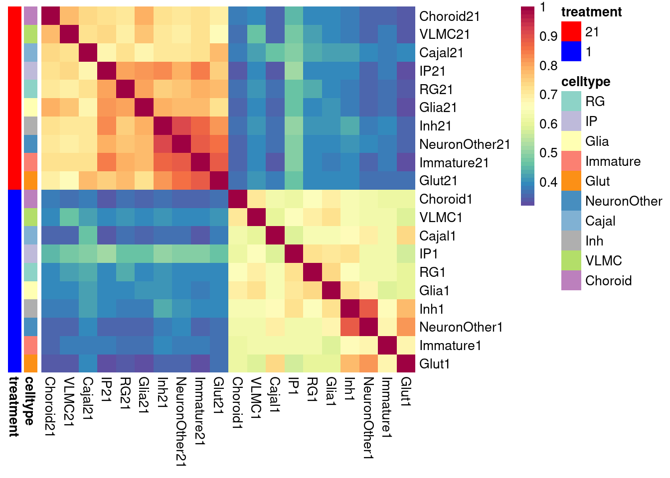
Version	Author	Date
e2547f5	Ben Umans	2025-02-24

# for logFC-constrained
labels <- data.frame(celltype=str_extract(rownames(shared.size.constrained), pattern = "[:alpha:]+"),
                     treatment=str_extract(rownames(shared.size.constrained), pattern = "[:digit:]+"))
rownames(labels) <- rownames(shared.size.constrained)

celltypeCol <- manual_palette_coarse
treatmentCol <- c("red", "blue")
names(treatmentCol) <- unique(labels$treatment)
annoCol <- list(celltype = celltypeCol,
                treatment = treatmentCol)

pheatmap(shared.size.constrained, col = colorRampPalette(rev(brewer.pal(11, "Spectral")))(50),
         border_color = NA,
         show_colnames = TRUE,
         treeheight_row = 0, treeheight_col = 0,
         annotation_row = labels,
         annotation_colors = annoCol, cluster_rows = FALSE, cluster_cols = FALSE
)

Past versions of unnamed-chunk-47-2.png

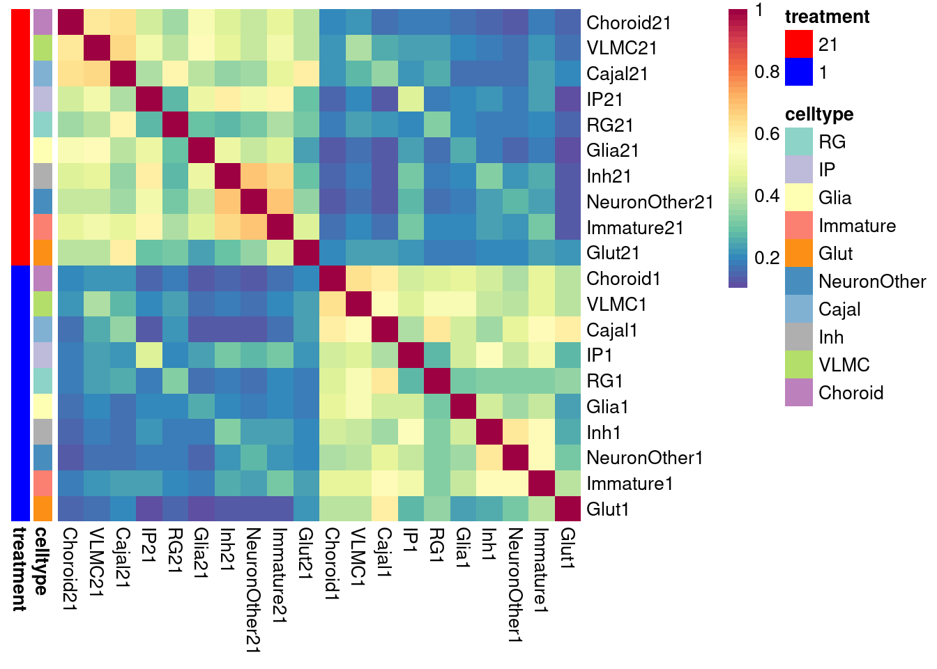
Version	Author	Date
e2547f5	Ben Umans	2025-02-24

Gene set enrichment

We used fgsea to compare differential expression results to annotated gene sets from MsigDB.

m_posterior <- readRDS(file="/project2/gilad/umans/oxygen_eqtl/output/mash_de/mashposterior_dataset9_fine_reharmonized_z3.RDS")

library(fgsea)
pathways_all <- gmtPathways('/project/gilad/umans/references/msigdb/h.all.v2023.1.Hs.symbols.gmt') 
# obtained from https://www.gsea-msigdb.org/gsea/msigdb/collections.jsp

Calculate a t-statistic for mash output, as very small lfsr significance metrics can skew fgsea results.

m_posterior$t <- m_posterior$PosteriorMean/m_posterior$PosteriorSD

Next, perform fgsea on each cell type/condition (ie, each column of this matrix).

for (i in colnames(m_posterior$t)){
  ranks <- m_posterior$t[, i]
  fgseaRes <- fgsea(pathways = pathways_all, 
                  stats    = ranks,
                  scoreType = "std",
                  eps = 0,
                  nproc = 5)
  all <- fgseaRes[order(abs(fgseaRes$pval), decreasing = FALSE),]
  write_tsv(all, file = paste0("/project2/gilad/umans/oxygen_eqtl/output/fgsea/", i, "_fgsea_all_reharmonized_fine.txt"), quote = "none", col_names = TRUE)
  rm(all, ranks, fgseaRes)
}

Plot p-values

combined_fgsea_all <- read_tsv(file = paste0("/project2/gilad/umans/oxygen_eqtl/output/fgsea/", colnames(m_posterior$t)[1], "_fgsea_all_reharmonized_fine.txt"), col_names = TRUE) %>% dplyr::select(pathway, !!colnames(m_posterior$t)[1] := padj)

Rows: 50 Columns: 8
── Column specification ────────────────────────────────────────────────────────
Delimiter: "\t"
chr (1): pathway
dbl (6): pval, padj, log2err, ES, NES, size
lgl (1): leadingEdge

ℹ Use `spec()` to retrieve the full column specification for this data.
ℹ Specify the column types or set `show_col_types = FALSE` to quiet this message.

for (i in colnames(m_posterior$t)[-1]){
  temp <- read_tsv(file = paste0("/project2/gilad/umans/oxygen_eqtl/output/fgsea/", i, "_fgsea_all_reharmonized_fine.txt"), col_names = TRUE) %>% dplyr::select(pathway, !!i := padj)
  combined_fgsea_all <- full_join(combined_fgsea_all, temp, by = "pathway")
  rm(temp)
}

Rows: 50 Columns: 8
── Column specification ────────────────────────────────────────────────────────
Delimiter: "\t"
chr (1): pathway
dbl (6): pval, padj, log2err, ES, NES, size
lgl (1): leadingEdge

ℹ Use `spec()` to retrieve the full column specification for this data.
ℹ Specify the column types or set `show_col_types = FALSE` to quiet this message.
Rows: 50 Columns: 8
── Column specification ────────────────────────────────────────────────────────
Delimiter: "\t"
chr (1): pathway
dbl (6): pval, padj, log2err, ES, NES, size
lgl (1): leadingEdge

ℹ Use `spec()` to retrieve the full column specification for this data.
ℹ Specify the column types or set `show_col_types = FALSE` to quiet this message.
Rows: 50 Columns: 8
── Column specification ────────────────────────────────────────────────────────
Delimiter: "\t"
chr (1): pathway
dbl (6): pval, padj, log2err, ES, NES, size
lgl (1): leadingEdge

ℹ Use `spec()` to retrieve the full column specification for this data.
ℹ Specify the column types or set `show_col_types = FALSE` to quiet this message.
Rows: 50 Columns: 8
── Column specification ────────────────────────────────────────────────────────
Delimiter: "\t"
chr (1): pathway
dbl (6): pval, padj, log2err, ES, NES, size
lgl (1): leadingEdge

ℹ Use `spec()` to retrieve the full column specification for this data.
ℹ Specify the column types or set `show_col_types = FALSE` to quiet this message.
Rows: 50 Columns: 8
── Column specification ────────────────────────────────────────────────────────
Delimiter: "\t"
chr (1): pathway
dbl (6): pval, padj, log2err, ES, NES, size
lgl (1): leadingEdge

ℹ Use `spec()` to retrieve the full column specification for this data.
ℹ Specify the column types or set `show_col_types = FALSE` to quiet this message.
Rows: 50 Columns: 8
── Column specification ────────────────────────────────────────────────────────
Delimiter: "\t"
chr (1): pathway
dbl (6): pval, padj, log2err, ES, NES, size
lgl (1): leadingEdge

ℹ Use `spec()` to retrieve the full column specification for this data.
ℹ Specify the column types or set `show_col_types = FALSE` to quiet this message.
Rows: 50 Columns: 8
── Column specification ────────────────────────────────────────────────────────
Delimiter: "\t"
chr (1): pathway
dbl (6): pval, padj, log2err, ES, NES, size
lgl (1): leadingEdge

ℹ Use `spec()` to retrieve the full column specification for this data.
ℹ Specify the column types or set `show_col_types = FALSE` to quiet this message.
Rows: 50 Columns: 8
── Column specification ────────────────────────────────────────────────────────
Delimiter: "\t"
chr (1): pathway
dbl (6): pval, padj, log2err, ES, NES, size
lgl (1): leadingEdge

ℹ Use `spec()` to retrieve the full column specification for this data.
ℹ Specify the column types or set `show_col_types = FALSE` to quiet this message.
Rows: 50 Columns: 8
── Column specification ────────────────────────────────────────────────────────
Delimiter: "\t"
chr (1): pathway
dbl (6): pval, padj, log2err, ES, NES, size
lgl (1): leadingEdge

ℹ Use `spec()` to retrieve the full column specification for this data.
ℹ Specify the column types or set `show_col_types = FALSE` to quiet this message.
Rows: 50 Columns: 8
── Column specification ────────────────────────────────────────────────────────
Delimiter: "\t"
chr (1): pathway
dbl (6): pval, padj, log2err, ES, NES, size
lgl (1): leadingEdge

ℹ Use `spec()` to retrieve the full column specification for this data.
ℹ Specify the column types or set `show_col_types = FALSE` to quiet this message.
Rows: 50 Columns: 8
── Column specification ────────────────────────────────────────────────────────
Delimiter: "\t"
chr (1): pathway
dbl (6): pval, padj, log2err, ES, NES, size
lgl (1): leadingEdge

ℹ Use `spec()` to retrieve the full column specification for this data.
ℹ Specify the column types or set `show_col_types = FALSE` to quiet this message.
Rows: 50 Columns: 8
── Column specification ────────────────────────────────────────────────────────
Delimiter: "\t"
chr (1): pathway
dbl (6): pval, padj, log2err, ES, NES, size
lgl (1): leadingEdge

ℹ Use `spec()` to retrieve the full column specification for this data.
ℹ Specify the column types or set `show_col_types = FALSE` to quiet this message.
Rows: 50 Columns: 8
── Column specification ────────────────────────────────────────────────────────
Delimiter: "\t"
chr (1): pathway
dbl (6): pval, padj, log2err, ES, NES, size
lgl (1): leadingEdge

ℹ Use `spec()` to retrieve the full column specification for this data.
ℹ Specify the column types or set `show_col_types = FALSE` to quiet this message.
Rows: 50 Columns: 8
── Column specification ────────────────────────────────────────────────────────
Delimiter: "\t"
chr (1): pathway
dbl (6): pval, padj, log2err, ES, NES, size
lgl (1): leadingEdge

ℹ Use `spec()` to retrieve the full column specification for this data.
ℹ Specify the column types or set `show_col_types = FALSE` to quiet this message.
Rows: 50 Columns: 8
── Column specification ────────────────────────────────────────────────────────
Delimiter: "\t"
chr (1): pathway
dbl (6): pval, padj, log2err, ES, NES, size
lgl (1): leadingEdge

ℹ Use `spec()` to retrieve the full column specification for this data.
ℹ Specify the column types or set `show_col_types = FALSE` to quiet this message.
Rows: 50 Columns: 8
── Column specification ────────────────────────────────────────────────────────
Delimiter: "\t"
chr (1): pathway
dbl (6): pval, padj, log2err, ES, NES, size
lgl (1): leadingEdge

ℹ Use `spec()` to retrieve the full column specification for this data.
ℹ Specify the column types or set `show_col_types = FALSE` to quiet this message.
Rows: 50 Columns: 8
── Column specification ────────────────────────────────────────────────────────
Delimiter: "\t"
chr (1): pathway
dbl (6): pval, padj, log2err, ES, NES, size
lgl (1): leadingEdge

ℹ Use `spec()` to retrieve the full column specification for this data.
ℹ Specify the column types or set `show_col_types = FALSE` to quiet this message.
Rows: 50 Columns: 8
── Column specification ────────────────────────────────────────────────────────
Delimiter: "\t"
chr (1): pathway
dbl (6): pval, padj, log2err, ES, NES, size
lgl (1): leadingEdge

ℹ Use `spec()` to retrieve the full column specification for this data.
ℹ Specify the column types or set `show_col_types = FALSE` to quiet this message.
Rows: 50 Columns: 8
── Column specification ────────────────────────────────────────────────────────
Delimiter: "\t"
chr (1): pathway
dbl (6): pval, padj, log2err, ES, NES, size
lgl (1): leadingEdge

ℹ Use `spec()` to retrieve the full column specification for this data.
ℹ Specify the column types or set `show_col_types = FALSE` to quiet this message.
Rows: 50 Columns: 8
── Column specification ────────────────────────────────────────────────────────
Delimiter: "\t"
chr (1): pathway
dbl (6): pval, padj, log2err, ES, NES, size
lgl (1): leadingEdge

ℹ Use `spec()` to retrieve the full column specification for this data.
ℹ Specify the column types or set `show_col_types = FALSE` to quiet this message.
Rows: 50 Columns: 8
── Column specification ────────────────────────────────────────────────────────
Delimiter: "\t"
chr (1): pathway
dbl (6): pval, padj, log2err, ES, NES, size
lgl (1): leadingEdge

ℹ Use `spec()` to retrieve the full column specification for this data.
ℹ Specify the column types or set `show_col_types = FALSE` to quiet this message.
Rows: 50 Columns: 8
── Column specification ────────────────────────────────────────────────────────
Delimiter: "\t"
chr (1): pathway
dbl (6): pval, padj, log2err, ES, NES, size
lgl (1): leadingEdge

ℹ Use `spec()` to retrieve the full column specification for this data.
ℹ Specify the column types or set `show_col_types = FALSE` to quiet this message.
Rows: 50 Columns: 8
── Column specification ────────────────────────────────────────────────────────
Delimiter: "\t"
chr (1): pathway
dbl (6): pval, padj, log2err, ES, NES, size
lgl (1): leadingEdge

ℹ Use `spec()` to retrieve the full column specification for this data.
ℹ Specify the column types or set `show_col_types = FALSE` to quiet this message.
Rows: 50 Columns: 8
── Column specification ────────────────────────────────────────────────────────
Delimiter: "\t"
chr (1): pathway
dbl (6): pval, padj, log2err, ES, NES, size
lgl (1): leadingEdge

ℹ Use `spec()` to retrieve the full column specification for this data.
ℹ Specify the column types or set `show_col_types = FALSE` to quiet this message.
Rows: 50 Columns: 8
── Column specification ────────────────────────────────────────────────────────
Delimiter: "\t"
chr (1): pathway
dbl (6): pval, padj, log2err, ES, NES, size
lgl (1): leadingEdge

ℹ Use `spec()` to retrieve the full column specification for this data.
ℹ Specify the column types or set `show_col_types = FALSE` to quiet this message.
Rows: 50 Columns: 8
── Column specification ────────────────────────────────────────────────────────
Delimiter: "\t"
chr (1): pathway
dbl (6): pval, padj, log2err, ES, NES, size
lgl (1): leadingEdge

ℹ Use `spec()` to retrieve the full column specification for this data.
ℹ Specify the column types or set `show_col_types = FALSE` to quiet this message.
Rows: 50 Columns: 8
── Column specification ────────────────────────────────────────────────────────
Delimiter: "\t"
chr (1): pathway
dbl (6): pval, padj, log2err, ES, NES, size
lgl (1): leadingEdge

ℹ Use `spec()` to retrieve the full column specification for this data.
ℹ Specify the column types or set `show_col_types = FALSE` to quiet this message.
Rows: 50 Columns: 8
── Column specification ────────────────────────────────────────────────────────
Delimiter: "\t"
chr (1): pathway
dbl (6): pval, padj, log2err, ES, NES, size
lgl (1): leadingEdge

ℹ Use `spec()` to retrieve the full column specification for this data.
ℹ Specify the column types or set `show_col_types = FALSE` to quiet this message.
Rows: 50 Columns: 8
── Column specification ────────────────────────────────────────────────────────
Delimiter: "\t"
chr (1): pathway
dbl (6): pval, padj, log2err, ES, NES, size
lgl (1): leadingEdge

ℹ Use `spec()` to retrieve the full column specification for this data.
ℹ Specify the column types or set `show_col_types = FALSE` to quiet this message.
Rows: 50 Columns: 8
── Column specification ────────────────────────────────────────────────────────
Delimiter: "\t"
chr (1): pathway
dbl (6): pval, padj, log2err, ES, NES, size
lgl (1): leadingEdge

ℹ Use `spec()` to retrieve the full column specification for this data.
ℹ Specify the column types or set `show_col_types = FALSE` to quiet this message.
Rows: 50 Columns: 8
── Column specification ────────────────────────────────────────────────────────
Delimiter: "\t"
chr (1): pathway
dbl (6): pval, padj, log2err, ES, NES, size
lgl (1): leadingEdge

ℹ Use `spec()` to retrieve the full column specification for this data.
ℹ Specify the column types or set `show_col_types = FALSE` to quiet this message.
Rows: 50 Columns: 8
── Column specification ────────────────────────────────────────────────────────
Delimiter: "\t"
chr (1): pathway
dbl (6): pval, padj, log2err, ES, NES, size
lgl (1): leadingEdge

ℹ Use `spec()` to retrieve the full column specification for this data.
ℹ Specify the column types or set `show_col_types = FALSE` to quiet this message.
Rows: 50 Columns: 8
── Column specification ────────────────────────────────────────────────────────
Delimiter: "\t"
chr (1): pathway
dbl (6): pval, padj, log2err, ES, NES, size
lgl (1): leadingEdge

ℹ Use `spec()` to retrieve the full column specification for this data.
ℹ Specify the column types or set `show_col_types = FALSE` to quiet this message.
Rows: 50 Columns: 8
── Column specification ────────────────────────────────────────────────────────
Delimiter: "\t"
chr (1): pathway
dbl (6): pval, padj, log2err, ES, NES, size
lgl (1): leadingEdge

ℹ Use `spec()` to retrieve the full column specification for this data.
ℹ Specify the column types or set `show_col_types = FALSE` to quiet this message.
Rows: 50 Columns: 8
── Column specification ────────────────────────────────────────────────────────
Delimiter: "\t"
chr (1): pathway
dbl (6): pval, padj, log2err, ES, NES, size
lgl (1): leadingEdge

ℹ Use `spec()` to retrieve the full column specification for this data.
ℹ Specify the column types or set `show_col_types = FALSE` to quiet this message.

combined_fgsea_all <- combined_fgsea_all %>% column_to_rownames(var = "pathway") 

significant_hallmark <- combined_fgsea_all %>% filter(if_any(everything(), ~ .<0.05)) %>% rownames()


labels <- data.frame(celltype=str_extract(colnames(combined_fgsea_all), pattern = "[:alpha:]+"),
                     treatment=str_extract(colnames(combined_fgsea_all), pattern = "[:digit:]+"))

rownames(labels) <- colnames(combined_fgsea_all)

celltypeCol <- manual_palette_fine
treatmentCol <- c("red", "blue")
names(treatmentCol) <- unique(labels$treatment)
annoCol <- list(celltype = celltypeCol,
                treatment = treatmentCol)

combined_fgsea_all <- combined_fgsea_all[, c("RGcycling21" , "RG21", "CorticalHem21", "IPcycling21", "IP21", "GliaProg21", "Immature21", "Glut21", "GlutNTS21", "NeuronOther21", "Cajal21",  "Inh21",  "InhThalamic21", "InhGNRH21",  "InhSST21", "InhMidbrain21", "VLMC21", "Choroid21", "RGcycling1" , "RG1", "CorticalHem1", "IPcycling1", "IP1", "GliaProg1", "Immature1", "Glut1", "GlutNTS1", "NeuronOther1", "Cajal1",  "Inh1",  "InhThalamic1", "InhGNRH1",  "InhSST1", "InhMidbrain1", "VLMC1", "Choroid1")]


# now use pheatmap to annotate
pheatmap(-log10(combined_fgsea_all), col = colorRampPalette(rev(brewer.pal(11, "Spectral")))(25),
         border_color = NA,
         show_colnames = TRUE,
         treeheight_row = 0, treeheight_col = 0,
         annotation_col = labels,
         annotation_colors = annoCol, cluster_cols = FALSE
         )

Past versions of unnamed-chunk-52-1.png

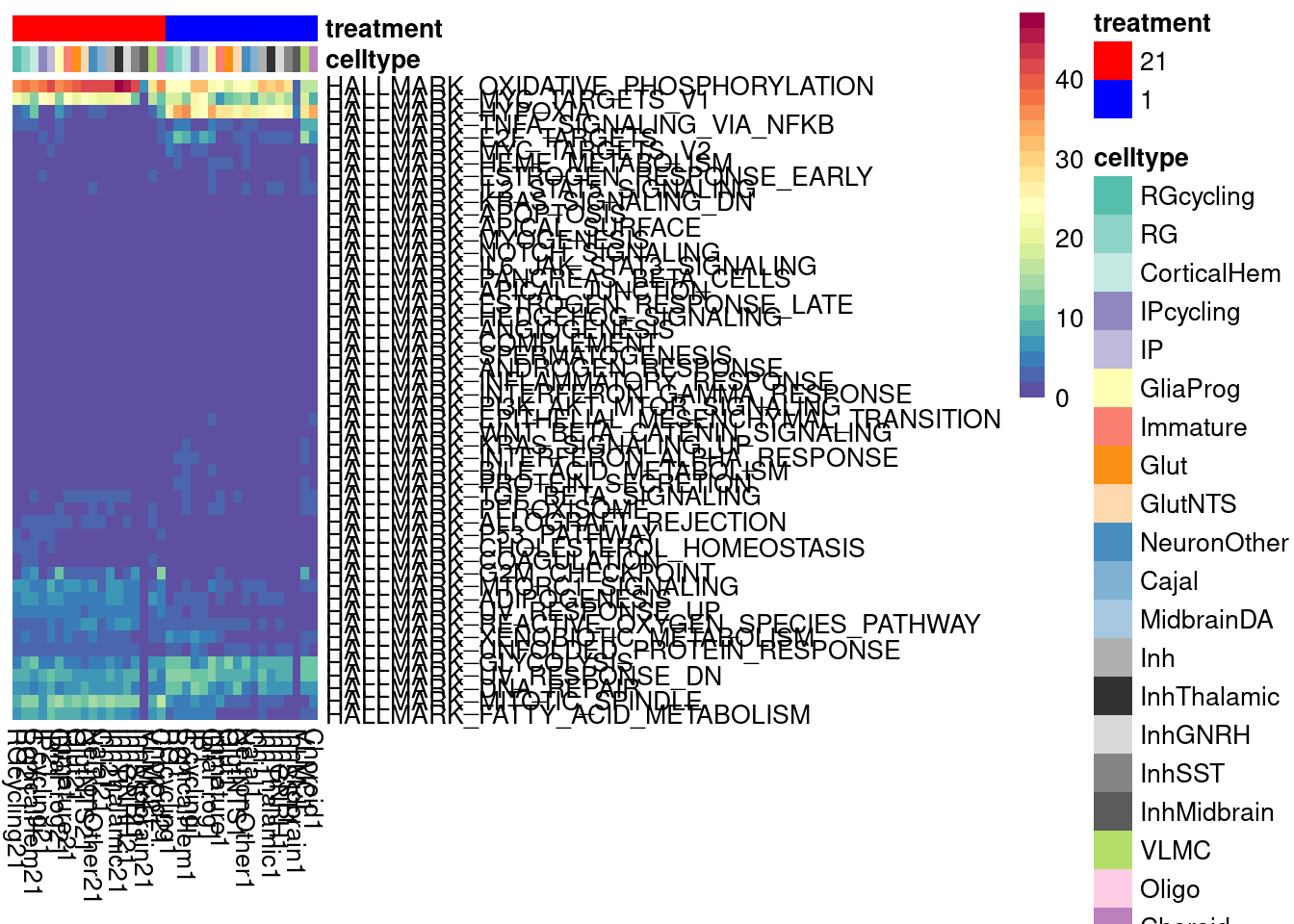
Version	Author	Date
e2547f5	Ben Umans	2025-02-24

rm(combined_fgsea_all)

Combine the output into a single matrix and plot the normalized effect sizes

combined_fgsea_all <- read_tsv(file = paste0("/project2/gilad/umans/oxygen_eqtl/output/fgsea/", colnames(m_posterior$t)[1], "_fgsea_all_reharmonized_fine.txt"), col_names = TRUE) %>% dplyr::select(pathway, !!colnames(m_posterior$t)[1] := NES)

Rows: 50 Columns: 8
── Column specification ────────────────────────────────────────────────────────
Delimiter: "\t"
chr (1): pathway
dbl (6): pval, padj, log2err, ES, NES, size
lgl (1): leadingEdge

ℹ Use `spec()` to retrieve the full column specification for this data.
ℹ Specify the column types or set `show_col_types = FALSE` to quiet this message.

for (i in colnames(m_posterior$t)[-1]){
  temp <- read_tsv(file = paste0("/project2/gilad/umans/oxygen_eqtl/output/fgsea/", i, "_fgsea_all_reharmonized_fine.txt"), col_names = TRUE) %>% dplyr::select(pathway, !!i := NES)
  combined_fgsea_all <- full_join(combined_fgsea_all, temp, by = "pathway")
  rm(temp)
}

Rows: 50 Columns: 8
── Column specification ────────────────────────────────────────────────────────
Delimiter: "\t"
chr (1): pathway
dbl (6): pval, padj, log2err, ES, NES, size
lgl (1): leadingEdge

ℹ Use `spec()` to retrieve the full column specification for this data.
ℹ Specify the column types or set `show_col_types = FALSE` to quiet this message.
Rows: 50 Columns: 8
── Column specification ────────────────────────────────────────────────────────
Delimiter: "\t"
chr (1): pathway
dbl (6): pval, padj, log2err, ES, NES, size
lgl (1): leadingEdge

ℹ Use `spec()` to retrieve the full column specification for this data.
ℹ Specify the column types or set `show_col_types = FALSE` to quiet this message.
Rows: 50 Columns: 8
── Column specification ────────────────────────────────────────────────────────
Delimiter: "\t"
chr (1): pathway
dbl (6): pval, padj, log2err, ES, NES, size
lgl (1): leadingEdge

ℹ Use `spec()` to retrieve the full column specification for this data.
ℹ Specify the column types or set `show_col_types = FALSE` to quiet this message.
Rows: 50 Columns: 8
── Column specification ────────────────────────────────────────────────────────
Delimiter: "\t"
chr (1): pathway
dbl (6): pval, padj, log2err, ES, NES, size
lgl (1): leadingEdge

ℹ Use `spec()` to retrieve the full column specification for this data.
ℹ Specify the column types or set `show_col_types = FALSE` to quiet this message.
Rows: 50 Columns: 8
── Column specification ────────────────────────────────────────────────────────
Delimiter: "\t"
chr (1): pathway
dbl (6): pval, padj, log2err, ES, NES, size
lgl (1): leadingEdge

ℹ Use `spec()` to retrieve the full column specification for this data.
ℹ Specify the column types or set `show_col_types = FALSE` to quiet this message.
Rows: 50 Columns: 8
── Column specification ────────────────────────────────────────────────────────
Delimiter: "\t"
chr (1): pathway
dbl (6): pval, padj, log2err, ES, NES, size
lgl (1): leadingEdge

ℹ Use `spec()` to retrieve the full column specification for this data.
ℹ Specify the column types or set `show_col_types = FALSE` to quiet this message.
Rows: 50 Columns: 8
── Column specification ────────────────────────────────────────────────────────
Delimiter: "\t"
chr (1): pathway
dbl (6): pval, padj, log2err, ES, NES, size
lgl (1): leadingEdge

ℹ Use `spec()` to retrieve the full column specification for this data.
ℹ Specify the column types or set `show_col_types = FALSE` to quiet this message.
Rows: 50 Columns: 8
── Column specification ────────────────────────────────────────────────────────
Delimiter: "\t"
chr (1): pathway
dbl (6): pval, padj, log2err, ES, NES, size
lgl (1): leadingEdge

ℹ Use `spec()` to retrieve the full column specification for this data.
ℹ Specify the column types or set `show_col_types = FALSE` to quiet this message.
Rows: 50 Columns: 8
── Column specification ────────────────────────────────────────────────────────
Delimiter: "\t"
chr (1): pathway
dbl (6): pval, padj, log2err, ES, NES, size
lgl (1): leadingEdge

ℹ Use `spec()` to retrieve the full column specification for this data.
ℹ Specify the column types or set `show_col_types = FALSE` to quiet this message.
Rows: 50 Columns: 8
── Column specification ────────────────────────────────────────────────────────
Delimiter: "\t"
chr (1): pathway
dbl (6): pval, padj, log2err, ES, NES, size
lgl (1): leadingEdge

ℹ Use `spec()` to retrieve the full column specification for this data.
ℹ Specify the column types or set `show_col_types = FALSE` to quiet this message.
Rows: 50 Columns: 8
── Column specification ────────────────────────────────────────────────────────
Delimiter: "\t"
chr (1): pathway
dbl (6): pval, padj, log2err, ES, NES, size
lgl (1): leadingEdge

ℹ Use `spec()` to retrieve the full column specification for this data.
ℹ Specify the column types or set `show_col_types = FALSE` to quiet this message.
Rows: 50 Columns: 8
── Column specification ────────────────────────────────────────────────────────
Delimiter: "\t"
chr (1): pathway
dbl (6): pval, padj, log2err, ES, NES, size
lgl (1): leadingEdge

ℹ Use `spec()` to retrieve the full column specification for this data.
ℹ Specify the column types or set `show_col_types = FALSE` to quiet this message.
Rows: 50 Columns: 8
── Column specification ────────────────────────────────────────────────────────
Delimiter: "\t"
chr (1): pathway
dbl (6): pval, padj, log2err, ES, NES, size
lgl (1): leadingEdge

ℹ Use `spec()` to retrieve the full column specification for this data.
ℹ Specify the column types or set `show_col_types = FALSE` to quiet this message.
Rows: 50 Columns: 8
── Column specification ────────────────────────────────────────────────────────
Delimiter: "\t"
chr (1): pathway
dbl (6): pval, padj, log2err, ES, NES, size
lgl (1): leadingEdge

ℹ Use `spec()` to retrieve the full column specification for this data.
ℹ Specify the column types or set `show_col_types = FALSE` to quiet this message.
Rows: 50 Columns: 8
── Column specification ────────────────────────────────────────────────────────
Delimiter: "\t"
chr (1): pathway
dbl (6): pval, padj, log2err, ES, NES, size
lgl (1): leadingEdge

ℹ Use `spec()` to retrieve the full column specification for this data.
ℹ Specify the column types or set `show_col_types = FALSE` to quiet this message.
Rows: 50 Columns: 8
── Column specification ────────────────────────────────────────────────────────
Delimiter: "\t"
chr (1): pathway
dbl (6): pval, padj, log2err, ES, NES, size
lgl (1): leadingEdge

ℹ Use `spec()` to retrieve the full column specification for this data.
ℹ Specify the column types or set `show_col_types = FALSE` to quiet this message.
Rows: 50 Columns: 8
── Column specification ────────────────────────────────────────────────────────
Delimiter: "\t"
chr (1): pathway
dbl (6): pval, padj, log2err, ES, NES, size
lgl (1): leadingEdge

ℹ Use `spec()` to retrieve the full column specification for this data.
ℹ Specify the column types or set `show_col_types = FALSE` to quiet this message.
Rows: 50 Columns: 8
── Column specification ────────────────────────────────────────────────────────
Delimiter: "\t"
chr (1): pathway
dbl (6): pval, padj, log2err, ES, NES, size
lgl (1): leadingEdge

ℹ Use `spec()` to retrieve the full column specification for this data.
ℹ Specify the column types or set `show_col_types = FALSE` to quiet this message.
Rows: 50 Columns: 8
── Column specification ────────────────────────────────────────────────────────
Delimiter: "\t"
chr (1): pathway
dbl (6): pval, padj, log2err, ES, NES, size
lgl (1): leadingEdge

ℹ Use `spec()` to retrieve the full column specification for this data.
ℹ Specify the column types or set `show_col_types = FALSE` to quiet this message.
Rows: 50 Columns: 8
── Column specification ────────────────────────────────────────────────────────
Delimiter: "\t"
chr (1): pathway
dbl (6): pval, padj, log2err, ES, NES, size
lgl (1): leadingEdge

ℹ Use `spec()` to retrieve the full column specification for this data.
ℹ Specify the column types or set `show_col_types = FALSE` to quiet this message.
Rows: 50 Columns: 8
── Column specification ────────────────────────────────────────────────────────
Delimiter: "\t"
chr (1): pathway
dbl (6): pval, padj, log2err, ES, NES, size
lgl (1): leadingEdge

ℹ Use `spec()` to retrieve the full column specification for this data.
ℹ Specify the column types or set `show_col_types = FALSE` to quiet this message.
Rows: 50 Columns: 8
── Column specification ────────────────────────────────────────────────────────
Delimiter: "\t"
chr (1): pathway
dbl (6): pval, padj, log2err, ES, NES, size
lgl (1): leadingEdge

ℹ Use `spec()` to retrieve the full column specification for this data.
ℹ Specify the column types or set `show_col_types = FALSE` to quiet this message.
Rows: 50 Columns: 8
── Column specification ────────────────────────────────────────────────────────
Delimiter: "\t"
chr (1): pathway
dbl (6): pval, padj, log2err, ES, NES, size
lgl (1): leadingEdge

ℹ Use `spec()` to retrieve the full column specification for this data.
ℹ Specify the column types or set `show_col_types = FALSE` to quiet this message.
Rows: 50 Columns: 8
── Column specification ────────────────────────────────────────────────────────
Delimiter: "\t"
chr (1): pathway
dbl (6): pval, padj, log2err, ES, NES, size
lgl (1): leadingEdge

ℹ Use `spec()` to retrieve the full column specification for this data.
ℹ Specify the column types or set `show_col_types = FALSE` to quiet this message.
Rows: 50 Columns: 8
── Column specification ────────────────────────────────────────────────────────
Delimiter: "\t"
chr (1): pathway
dbl (6): pval, padj, log2err, ES, NES, size
lgl (1): leadingEdge

ℹ Use `spec()` to retrieve the full column specification for this data.
ℹ Specify the column types or set `show_col_types = FALSE` to quiet this message.
Rows: 50 Columns: 8
── Column specification ────────────────────────────────────────────────────────
Delimiter: "\t"
chr (1): pathway
dbl (6): pval, padj, log2err, ES, NES, size
lgl (1): leadingEdge

ℹ Use `spec()` to retrieve the full column specification for this data.
ℹ Specify the column types or set `show_col_types = FALSE` to quiet this message.
Rows: 50 Columns: 8
── Column specification ────────────────────────────────────────────────────────
Delimiter: "\t"
chr (1): pathway
dbl (6): pval, padj, log2err, ES, NES, size
lgl (1): leadingEdge

ℹ Use `spec()` to retrieve the full column specification for this data.
ℹ Specify the column types or set `show_col_types = FALSE` to quiet this message.
Rows: 50 Columns: 8
── Column specification ────────────────────────────────────────────────────────
Delimiter: "\t"
chr (1): pathway
dbl (6): pval, padj, log2err, ES, NES, size
lgl (1): leadingEdge

ℹ Use `spec()` to retrieve the full column specification for this data.
ℹ Specify the column types or set `show_col_types = FALSE` to quiet this message.
Rows: 50 Columns: 8
── Column specification ────────────────────────────────────────────────────────
Delimiter: "\t"
chr (1): pathway
dbl (6): pval, padj, log2err, ES, NES, size
lgl (1): leadingEdge

ℹ Use `spec()` to retrieve the full column specification for this data.
ℹ Specify the column types or set `show_col_types = FALSE` to quiet this message.
Rows: 50 Columns: 8
── Column specification ────────────────────────────────────────────────────────
Delimiter: "\t"
chr (1): pathway
dbl (6): pval, padj, log2err, ES, NES, size
lgl (1): leadingEdge

ℹ Use `spec()` to retrieve the full column specification for this data.
ℹ Specify the column types or set `show_col_types = FALSE` to quiet this message.
Rows: 50 Columns: 8
── Column specification ────────────────────────────────────────────────────────
Delimiter: "\t"
chr (1): pathway
dbl (6): pval, padj, log2err, ES, NES, size
lgl (1): leadingEdge

ℹ Use `spec()` to retrieve the full column specification for this data.
ℹ Specify the column types or set `show_col_types = FALSE` to quiet this message.
Rows: 50 Columns: 8
── Column specification ────────────────────────────────────────────────────────
Delimiter: "\t"
chr (1): pathway
dbl (6): pval, padj, log2err, ES, NES, size
lgl (1): leadingEdge

ℹ Use `spec()` to retrieve the full column specification for this data.
ℹ Specify the column types or set `show_col_types = FALSE` to quiet this message.
Rows: 50 Columns: 8
── Column specification ────────────────────────────────────────────────────────
Delimiter: "\t"
chr (1): pathway
dbl (6): pval, padj, log2err, ES, NES, size
lgl (1): leadingEdge

ℹ Use `spec()` to retrieve the full column specification for this data.
ℹ Specify the column types or set `show_col_types = FALSE` to quiet this message.
Rows: 50 Columns: 8
── Column specification ────────────────────────────────────────────────────────
Delimiter: "\t"
chr (1): pathway
dbl (6): pval, padj, log2err, ES, NES, size
lgl (1): leadingEdge

ℹ Use `spec()` to retrieve the full column specification for this data.
ℹ Specify the column types or set `show_col_types = FALSE` to quiet this message.
Rows: 50 Columns: 8
── Column specification ────────────────────────────────────────────────────────
Delimiter: "\t"
chr (1): pathway
dbl (6): pval, padj, log2err, ES, NES, size
lgl (1): leadingEdge

ℹ Use `spec()` to retrieve the full column specification for this data.
ℹ Specify the column types or set `show_col_types = FALSE` to quiet this message.

combined_fgsea_all <- combined_fgsea_all %>% 
  filter(pathway %in% significant_hallmark) %>%
  column_to_rownames(var = "pathway")


labels <- data.frame(celltype=str_extract(colnames(combined_fgsea_all), pattern = "[:alpha:]+"),
                     treatment=str_extract(colnames(combined_fgsea_all), pattern = "[:digit:]+"))

rownames(labels) <- colnames(combined_fgsea_all)

celltypeCol <- manual_palette_fine
treatmentCol <- c("red", "blue")
names(treatmentCol) <- unique(labels$treatment)
annoCol <- list(celltype = celltypeCol,
                treatment = treatmentCol)

combined_fgsea_all <- combined_fgsea_all[, c("RGcycling21" , "RG21", "CorticalHem21", "IPcycling21", "IP21", "GliaProg21", "Immature21", "Glut21", "GlutNTS21", "NeuronOther21", "Cajal21",  "Inh21",  "InhThalamic21", "InhGNRH21",  "InhSST21", "InhMidbrain21", "VLMC21", "Choroid21", "RGcycling1" , "RG1", "CorticalHem1", "IPcycling1", "IP1", "GliaProg1", "Immature1", "Glut1", "GlutNTS1", "NeuronOther1", "Cajal1",  "Inh1",  "InhThalamic1", "InhGNRH1",  "InhSST1", "InhMidbrain1", "VLMC1", "Choroid1")]


# now use pheatmap to annotate
pheatmap(combined_fgsea_all, col = colorRampPalette(rev(brewer.pal(11, "Spectral")))(25),
         border_color = NA,
         show_colnames = TRUE,
         treeheight_row = 0, treeheight_col = 0,
         annotation_col = labels,
         annotation_colors = annoCol, cluster_cols = FALSE
         )

Past versions of unnamed-chunk-53-1.png

Version	Author	Date
e2547f5	Ben Umans	2025-02-24
f0eaf05	Ben Umans	2024-09-05

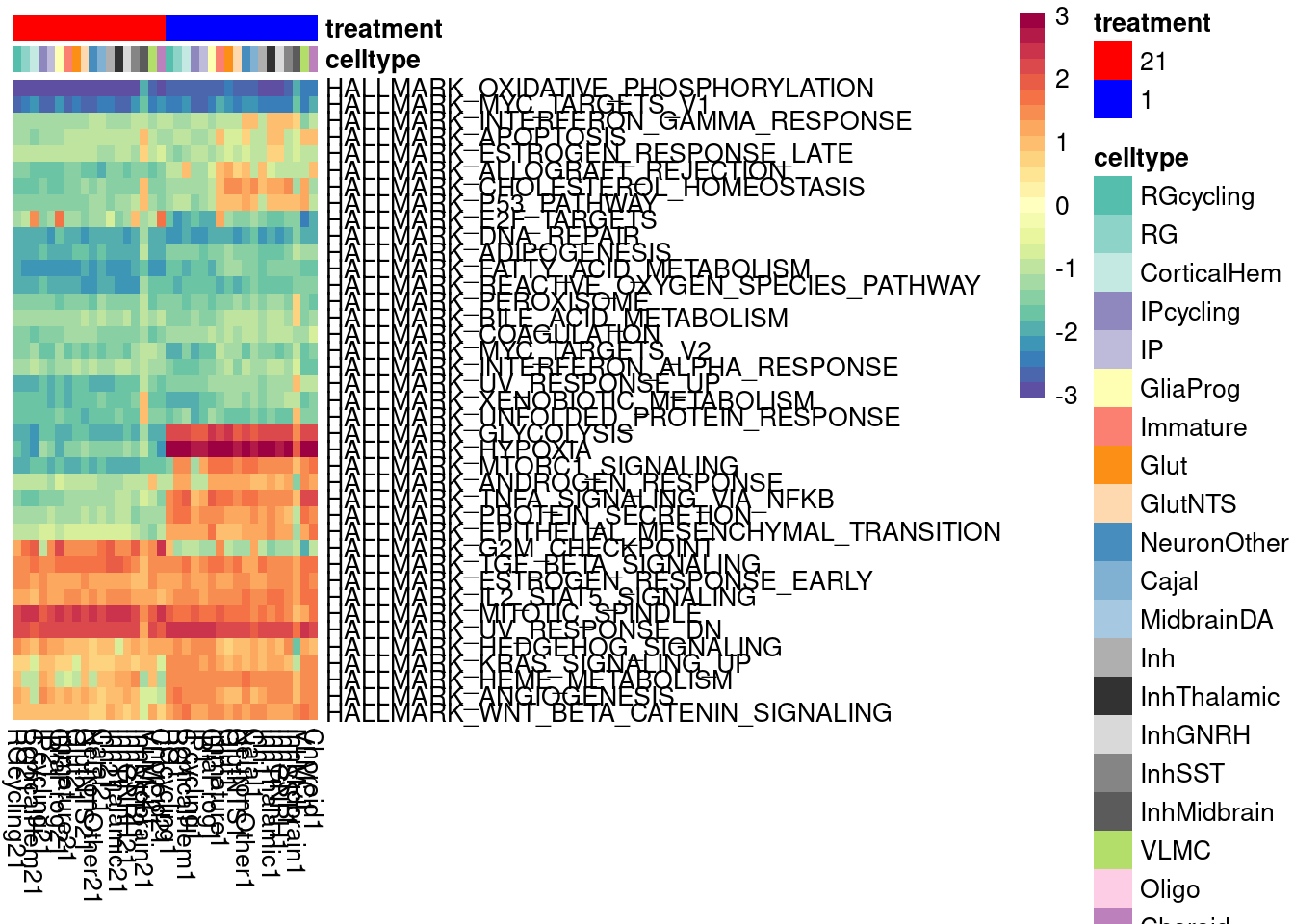
rm(combined_fgsea_all, m_posterior)

Gene set enrichment, coarse cell classification:

m_posterior <- readRDS(file="/project2/gilad/umans/oxygen_eqtl/output/mash_de/mashposterior_dataset9_coarse_reharmonized_z3.RDS")
m_posterior$t <- m_posterior$PosteriorMean/m_posterior$PosteriorSD

Next, perform fgsea on each cell type/condition (ie, each column of this matrix).

for (i in colnames(m_posterior$t)){
  ranks <- m_posterior$t[, i]
  fgseaRes <- fgsea(pathways = pathways_all, 
                    stats    = ranks,
                    scoreType = "std",
                    eps = 0,
                    nproc = 5)
  all <- fgseaRes[order(abs(fgseaRes$pval), decreasing = FALSE),]
  write_tsv(all, file = paste0("/project2/gilad/umans/oxygen_eqtl/output/fgsea/", i, "_fgsea_all_reharmonized_coarse.txt"), quote = "none", col_names = TRUE)
  rm(all, ranks, fgseaRes)
}

Plot p-values

combined_fgsea_all <- read_tsv(file = paste0("/project2/gilad/umans/oxygen_eqtl/output/fgsea/", colnames(m_posterior$t)[1], "_fgsea_all_reharmonized_coarse.txt"), col_names = TRUE) %>% dplyr::select(pathway, !!colnames(m_posterior$t)[1] := padj)

Rows: 50 Columns: 8
── Column specification ────────────────────────────────────────────────────────
Delimiter: "\t"
chr (1): pathway
dbl (6): pval, padj, log2err, ES, NES, size
lgl (1): leadingEdge

ℹ Use `spec()` to retrieve the full column specification for this data.
ℹ Specify the column types or set `show_col_types = FALSE` to quiet this message.

for (i in colnames(m_posterior$t)[-1]){
  temp <- read_tsv(file = paste0("/project2/gilad/umans/oxygen_eqtl/output/fgsea/", i, "_fgsea_all_reharmonized_coarse.txt"), col_names = TRUE) %>% dplyr::select(pathway, !!i := padj)
  combined_fgsea_all <- full_join(combined_fgsea_all, temp, by = "pathway")
  rm(temp)
}

Rows: 50 Columns: 8
── Column specification ────────────────────────────────────────────────────────
Delimiter: "\t"
chr (1): pathway
dbl (6): pval, padj, log2err, ES, NES, size
lgl (1): leadingEdge

ℹ Use `spec()` to retrieve the full column specification for this data.
ℹ Specify the column types or set `show_col_types = FALSE` to quiet this message.
Rows: 50 Columns: 8
── Column specification ────────────────────────────────────────────────────────
Delimiter: "\t"
chr (1): pathway
dbl (6): pval, padj, log2err, ES, NES, size
lgl (1): leadingEdge

ℹ Use `spec()` to retrieve the full column specification for this data.
ℹ Specify the column types or set `show_col_types = FALSE` to quiet this message.
Rows: 50 Columns: 8
── Column specification ────────────────────────────────────────────────────────
Delimiter: "\t"
chr (1): pathway
dbl (6): pval, padj, log2err, ES, NES, size
lgl (1): leadingEdge

ℹ Use `spec()` to retrieve the full column specification for this data.
ℹ Specify the column types or set `show_col_types = FALSE` to quiet this message.
Rows: 50 Columns: 8
── Column specification ────────────────────────────────────────────────────────
Delimiter: "\t"
chr (1): pathway
dbl (6): pval, padj, log2err, ES, NES, size
lgl (1): leadingEdge

ℹ Use `spec()` to retrieve the full column specification for this data.
ℹ Specify the column types or set `show_col_types = FALSE` to quiet this message.
Rows: 50 Columns: 8
── Column specification ────────────────────────────────────────────────────────
Delimiter: "\t"
chr (1): pathway
dbl (6): pval, padj, log2err, ES, NES, size
lgl (1): leadingEdge

ℹ Use `spec()` to retrieve the full column specification for this data.
ℹ Specify the column types or set `show_col_types = FALSE` to quiet this message.
Rows: 50 Columns: 8
── Column specification ────────────────────────────────────────────────────────
Delimiter: "\t"
chr (1): pathway
dbl (6): pval, padj, log2err, ES, NES, size
lgl (1): leadingEdge

ℹ Use `spec()` to retrieve the full column specification for this data.
ℹ Specify the column types or set `show_col_types = FALSE` to quiet this message.
Rows: 50 Columns: 8
── Column specification ────────────────────────────────────────────────────────
Delimiter: "\t"
chr (1): pathway
dbl (6): pval, padj, log2err, ES, NES, size
lgl (1): leadingEdge

ℹ Use `spec()` to retrieve the full column specification for this data.
ℹ Specify the column types or set `show_col_types = FALSE` to quiet this message.
Rows: 50 Columns: 8
── Column specification ────────────────────────────────────────────────────────
Delimiter: "\t"
chr (1): pathway
dbl (6): pval, padj, log2err, ES, NES, size
lgl (1): leadingEdge

ℹ Use `spec()` to retrieve the full column specification for this data.
ℹ Specify the column types or set `show_col_types = FALSE` to quiet this message.
Rows: 50 Columns: 8
── Column specification ────────────────────────────────────────────────────────
Delimiter: "\t"
chr (1): pathway
dbl (6): pval, padj, log2err, ES, NES, size
lgl (1): leadingEdge

ℹ Use `spec()` to retrieve the full column specification for this data.
ℹ Specify the column types or set `show_col_types = FALSE` to quiet this message.
Rows: 50 Columns: 8
── Column specification ────────────────────────────────────────────────────────
Delimiter: "\t"
chr (1): pathway
dbl (6): pval, padj, log2err, ES, NES, size
lgl (1): leadingEdge

ℹ Use `spec()` to retrieve the full column specification for this data.
ℹ Specify the column types or set `show_col_types = FALSE` to quiet this message.
Rows: 50 Columns: 8
── Column specification ────────────────────────────────────────────────────────
Delimiter: "\t"
chr (1): pathway
dbl (6): pval, padj, log2err, ES, NES, size
lgl (1): leadingEdge

ℹ Use `spec()` to retrieve the full column specification for this data.
ℹ Specify the column types or set `show_col_types = FALSE` to quiet this message.
Rows: 50 Columns: 8
── Column specification ────────────────────────────────────────────────────────
Delimiter: "\t"
chr (1): pathway
dbl (6): pval, padj, log2err, ES, NES, size
lgl (1): leadingEdge

ℹ Use `spec()` to retrieve the full column specification for this data.
ℹ Specify the column types or set `show_col_types = FALSE` to quiet this message.
Rows: 50 Columns: 8
── Column specification ────────────────────────────────────────────────────────
Delimiter: "\t"
chr (1): pathway
dbl (6): pval, padj, log2err, ES, NES, size
lgl (1): leadingEdge

ℹ Use `spec()` to retrieve the full column specification for this data.
ℹ Specify the column types or set `show_col_types = FALSE` to quiet this message.
Rows: 50 Columns: 8
── Column specification ────────────────────────────────────────────────────────
Delimiter: "\t"
chr (1): pathway
dbl (6): pval, padj, log2err, ES, NES, size
lgl (1): leadingEdge

ℹ Use `spec()` to retrieve the full column specification for this data.
ℹ Specify the column types or set `show_col_types = FALSE` to quiet this message.
Rows: 50 Columns: 8
── Column specification ────────────────────────────────────────────────────────
Delimiter: "\t"
chr (1): pathway
dbl (6): pval, padj, log2err, ES, NES, size
lgl (1): leadingEdge

ℹ Use `spec()` to retrieve the full column specification for this data.
ℹ Specify the column types or set `show_col_types = FALSE` to quiet this message.
Rows: 50 Columns: 8
── Column specification ────────────────────────────────────────────────────────
Delimiter: "\t"
chr (1): pathway
dbl (6): pval, padj, log2err, ES, NES, size
lgl (1): leadingEdge

ℹ Use `spec()` to retrieve the full column specification for this data.
ℹ Specify the column types or set `show_col_types = FALSE` to quiet this message.
Rows: 50 Columns: 8
── Column specification ────────────────────────────────────────────────────────
Delimiter: "\t"
chr (1): pathway
dbl (6): pval, padj, log2err, ES, NES, size
lgl (1): leadingEdge

ℹ Use `spec()` to retrieve the full column specification for this data.
ℹ Specify the column types or set `show_col_types = FALSE` to quiet this message.
Rows: 50 Columns: 8
── Column specification ────────────────────────────────────────────────────────
Delimiter: "\t"
chr (1): pathway
dbl (6): pval, padj, log2err, ES, NES, size
lgl (1): leadingEdge

ℹ Use `spec()` to retrieve the full column specification for this data.
ℹ Specify the column types or set `show_col_types = FALSE` to quiet this message.
Rows: 50 Columns: 8
── Column specification ────────────────────────────────────────────────────────
Delimiter: "\t"
chr (1): pathway
dbl (6): pval, padj, log2err, ES, NES, size
lgl (1): leadingEdge

ℹ Use `spec()` to retrieve the full column specification for this data.
ℹ Specify the column types or set `show_col_types = FALSE` to quiet this message.

combined_fgsea_all <- combined_fgsea_all %>% column_to_rownames(var = "pathway") 

significant_hallmark_coarse <- combined_fgsea_all %>% filter(if_any(everything(), ~ .<0.05)) %>% rownames()


labels <- data.frame(celltype=str_extract(colnames(combined_fgsea_all), pattern = "[:alpha:]+"),
                     treatment=str_extract(colnames(combined_fgsea_all), pattern = "[:digit:]+"))

rownames(labels) <- colnames(combined_fgsea_all)

celltypeCol <- manual_palette_coarse
treatmentCol <- c("red", "blue")
names(treatmentCol) <- unique(labels$treatment)
annoCol <- list(celltype = celltypeCol,
                treatment = treatmentCol)

combined_fgsea_all <- combined_fgsea_all[, c("RG21", "IP21", "Glia21", "Immature21", "Glut21", "NeuronOther21", "Cajal21",  "Inh21", "VLMC21", "Choroid21", "RG1", "IP1", "Glia1", "Immature1", "Glut1","NeuronOther1", "Cajal1",  "Inh1", "VLMC1", "Choroid1")]


# now use pheatmap to annotate
pheatmap(-log10(combined_fgsea_all), col = colorRampPalette(rev(brewer.pal(11, "Spectral")))(25),
         border_color = NA,
         show_colnames = TRUE,
         treeheight_row = 0, treeheight_col = 0,
         annotation_col = labels,
         annotation_colors = annoCol, cluster_cols = FALSE
         )

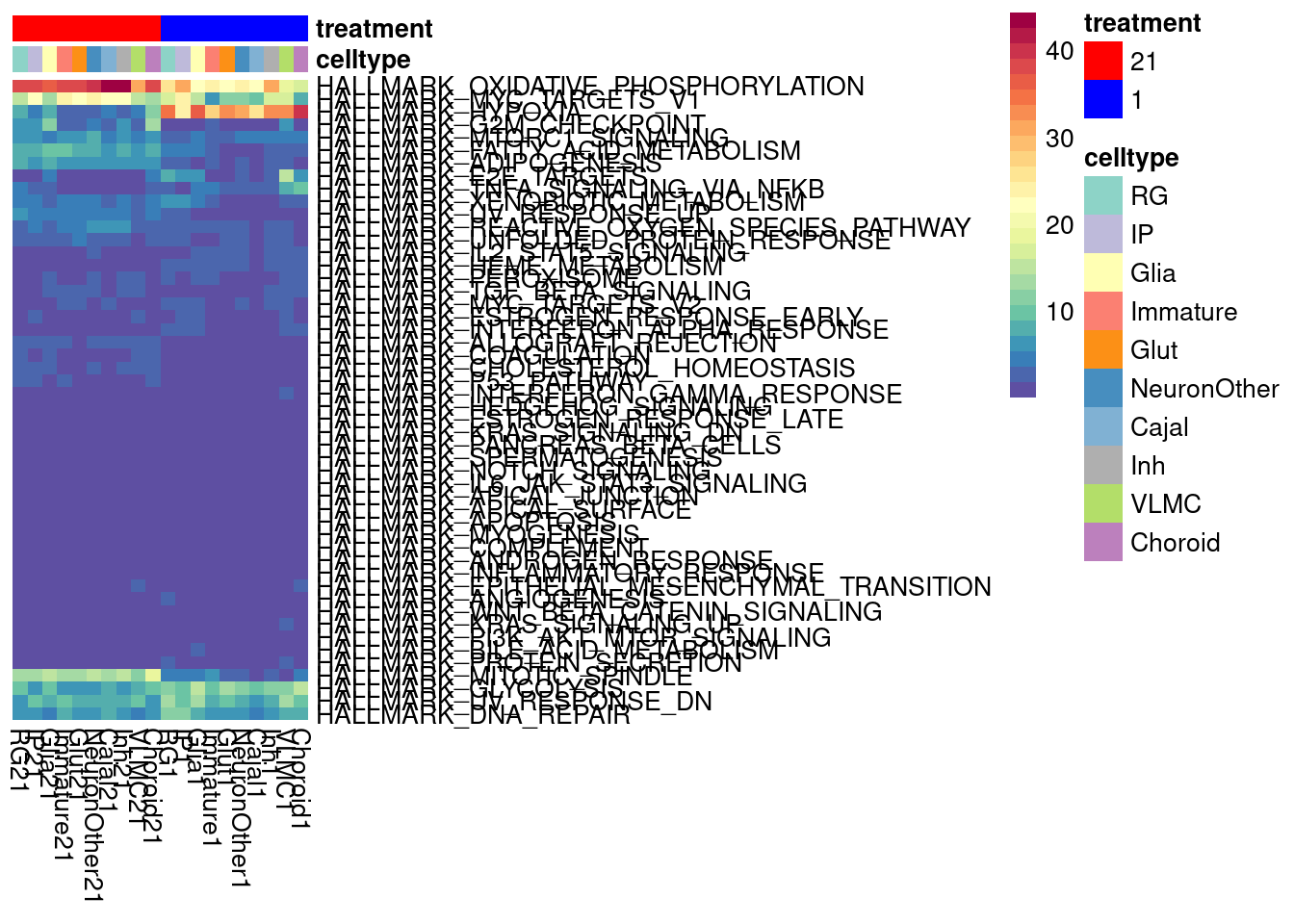
rm(combined_fgsea_all)

Combine the output into a single matrix and plot the normalized effect sizes

combined_fgsea_all <- read_tsv(file = paste0("/project2/gilad/umans/oxygen_eqtl/output/fgsea/", colnames(m_posterior$t)[1], "_fgsea_all_reharmonized_coarse.txt"), col_names = TRUE) %>% dplyr::select(pathway, !!colnames(m_posterior$t)[1] := NES)

Rows: 50 Columns: 8
── Column specification ────────────────────────────────────────────────────────
Delimiter: "\t"
chr (1): pathway
dbl (6): pval, padj, log2err, ES, NES, size
lgl (1): leadingEdge

ℹ Use `spec()` to retrieve the full column specification for this data.
ℹ Specify the column types or set `show_col_types = FALSE` to quiet this message.

for (i in colnames(m_posterior$t)[-1]){
  temp <- read_tsv(file = paste0("/project2/gilad/umans/oxygen_eqtl/output/fgsea/", i, "_fgsea_all_reharmonized_coarse.txt"), col_names = TRUE) %>% dplyr::select(pathway, !!i := NES)
  combined_fgsea_all <- full_join(combined_fgsea_all, temp, by = "pathway")
  rm(temp)
}

Rows: 50 Columns: 8
── Column specification ────────────────────────────────────────────────────────
Delimiter: "\t"
chr (1): pathway
dbl (6): pval, padj, log2err, ES, NES, size
lgl (1): leadingEdge

ℹ Use `spec()` to retrieve the full column specification for this data.
ℹ Specify the column types or set `show_col_types = FALSE` to quiet this message.
Rows: 50 Columns: 8
── Column specification ────────────────────────────────────────────────────────
Delimiter: "\t"
chr (1): pathway
dbl (6): pval, padj, log2err, ES, NES, size
lgl (1): leadingEdge

ℹ Use `spec()` to retrieve the full column specification for this data.
ℹ Specify the column types or set `show_col_types = FALSE` to quiet this message.
Rows: 50 Columns: 8
── Column specification ────────────────────────────────────────────────────────
Delimiter: "\t"
chr (1): pathway
dbl (6): pval, padj, log2err, ES, NES, size
lgl (1): leadingEdge

ℹ Use `spec()` to retrieve the full column specification for this data.
ℹ Specify the column types or set `show_col_types = FALSE` to quiet this message.
Rows: 50 Columns: 8
── Column specification ────────────────────────────────────────────────────────
Delimiter: "\t"
chr (1): pathway
dbl (6): pval, padj, log2err, ES, NES, size
lgl (1): leadingEdge

ℹ Use `spec()` to retrieve the full column specification for this data.
ℹ Specify the column types or set `show_col_types = FALSE` to quiet this message.
Rows: 50 Columns: 8
── Column specification ────────────────────────────────────────────────────────
Delimiter: "\t"
chr (1): pathway
dbl (6): pval, padj, log2err, ES, NES, size
lgl (1): leadingEdge

ℹ Use `spec()` to retrieve the full column specification for this data.
ℹ Specify the column types or set `show_col_types = FALSE` to quiet this message.
Rows: 50 Columns: 8
── Column specification ────────────────────────────────────────────────────────
Delimiter: "\t"
chr (1): pathway
dbl (6): pval, padj, log2err, ES, NES, size
lgl (1): leadingEdge

ℹ Use `spec()` to retrieve the full column specification for this data.
ℹ Specify the column types or set `show_col_types = FALSE` to quiet this message.
Rows: 50 Columns: 8
── Column specification ────────────────────────────────────────────────────────
Delimiter: "\t"
chr (1): pathway
dbl (6): pval, padj, log2err, ES, NES, size
lgl (1): leadingEdge

ℹ Use `spec()` to retrieve the full column specification for this data.
ℹ Specify the column types or set `show_col_types = FALSE` to quiet this message.
Rows: 50 Columns: 8
── Column specification ────────────────────────────────────────────────────────
Delimiter: "\t"
chr (1): pathway
dbl (6): pval, padj, log2err, ES, NES, size
lgl (1): leadingEdge

ℹ Use `spec()` to retrieve the full column specification for this data.
ℹ Specify the column types or set `show_col_types = FALSE` to quiet this message.
Rows: 50 Columns: 8
── Column specification ────────────────────────────────────────────────────────
Delimiter: "\t"
chr (1): pathway
dbl (6): pval, padj, log2err, ES, NES, size
lgl (1): leadingEdge

ℹ Use `spec()` to retrieve the full column specification for this data.
ℹ Specify the column types or set `show_col_types = FALSE` to quiet this message.
Rows: 50 Columns: 8
── Column specification ────────────────────────────────────────────────────────
Delimiter: "\t"
chr (1): pathway
dbl (6): pval, padj, log2err, ES, NES, size
lgl (1): leadingEdge

ℹ Use `spec()` to retrieve the full column specification for this data.
ℹ Specify the column types or set `show_col_types = FALSE` to quiet this message.
Rows: 50 Columns: 8
── Column specification ────────────────────────────────────────────────────────
Delimiter: "\t"
chr (1): pathway
dbl (6): pval, padj, log2err, ES, NES, size
lgl (1): leadingEdge

ℹ Use `spec()` to retrieve the full column specification for this data.
ℹ Specify the column types or set `show_col_types = FALSE` to quiet this message.
Rows: 50 Columns: 8
── Column specification ────────────────────────────────────────────────────────
Delimiter: "\t"
chr (1): pathway
dbl (6): pval, padj, log2err, ES, NES, size
lgl (1): leadingEdge

ℹ Use `spec()` to retrieve the full column specification for this data.
ℹ Specify the column types or set `show_col_types = FALSE` to quiet this message.
Rows: 50 Columns: 8
── Column specification ────────────────────────────────────────────────────────
Delimiter: "\t"
chr (1): pathway
dbl (6): pval, padj, log2err, ES, NES, size
lgl (1): leadingEdge

ℹ Use `spec()` to retrieve the full column specification for this data.
ℹ Specify the column types or set `show_col_types = FALSE` to quiet this message.
Rows: 50 Columns: 8
── Column specification ────────────────────────────────────────────────────────
Delimiter: "\t"
chr (1): pathway
dbl (6): pval, padj, log2err, ES, NES, size
lgl (1): leadingEdge

ℹ Use `spec()` to retrieve the full column specification for this data.
ℹ Specify the column types or set `show_col_types = FALSE` to quiet this message.
Rows: 50 Columns: 8
── Column specification ────────────────────────────────────────────────────────
Delimiter: "\t"
chr (1): pathway
dbl (6): pval, padj, log2err, ES, NES, size
lgl (1): leadingEdge

ℹ Use `spec()` to retrieve the full column specification for this data.
ℹ Specify the column types or set `show_col_types = FALSE` to quiet this message.
Rows: 50 Columns: 8
── Column specification ────────────────────────────────────────────────────────
Delimiter: "\t"
chr (1): pathway
dbl (6): pval, padj, log2err, ES, NES, size
lgl (1): leadingEdge

ℹ Use `spec()` to retrieve the full column specification for this data.
ℹ Specify the column types or set `show_col_types = FALSE` to quiet this message.
Rows: 50 Columns: 8
── Column specification ────────────────────────────────────────────────────────
Delimiter: "\t"
chr (1): pathway
dbl (6): pval, padj, log2err, ES, NES, size
lgl (1): leadingEdge

ℹ Use `spec()` to retrieve the full column specification for this data.
ℹ Specify the column types or set `show_col_types = FALSE` to quiet this message.
Rows: 50 Columns: 8
── Column specification ────────────────────────────────────────────────────────
Delimiter: "\t"
chr (1): pathway
dbl (6): pval, padj, log2err, ES, NES, size
lgl (1): leadingEdge

ℹ Use `spec()` to retrieve the full column specification for this data.
ℹ Specify the column types or set `show_col_types = FALSE` to quiet this message.
Rows: 50 Columns: 8
── Column specification ────────────────────────────────────────────────────────
Delimiter: "\t"
chr (1): pathway
dbl (6): pval, padj, log2err, ES, NES, size
lgl (1): leadingEdge

ℹ Use `spec()` to retrieve the full column specification for this data.
ℹ Specify the column types or set `show_col_types = FALSE` to quiet this message.

combined_fgsea_all <- combined_fgsea_all %>%
  filter(pathway %in% significant_hallmark_coarse) %>% 
  column_to_rownames(var = "pathway")


labels <- data.frame(celltype=str_extract(colnames(combined_fgsea_all), pattern = "[:alpha:]+"),
                     treatment=str_extract(colnames(combined_fgsea_all), pattern = "[:digit:]+"))

rownames(labels) <- colnames(combined_fgsea_all)

celltypeCol <- manual_palette_coarse
treatmentCol <- c("red", "blue")
names(treatmentCol) <- unique(labels$treatment)
annoCol <- list(celltype = celltypeCol,
                treatment = treatmentCol)

combined_fgsea_all <- combined_fgsea_all[, c( "RG21", "IP21", "Glia21", "Immature21", "Glut21", "NeuronOther21", "Cajal21",  "Inh21", "VLMC21", "Choroid21", "RG1", "IP1", "Glia1", "Immature1", "Glut1","NeuronOther1", "Cajal1",  "Inh1", "VLMC1", "Choroid1")]


# now use pheatmap to annotate
pheatmap(combined_fgsea_all, col = colorRampPalette(rev(brewer.pal(11, "Spectral")))(25),
         border_color = NA,
         show_colnames = TRUE,
         treeheight_row = 0, treeheight_col = 0,
         annotation_col = labels,
         annotation_colors = annoCol, cluster_cols = FALSE
)

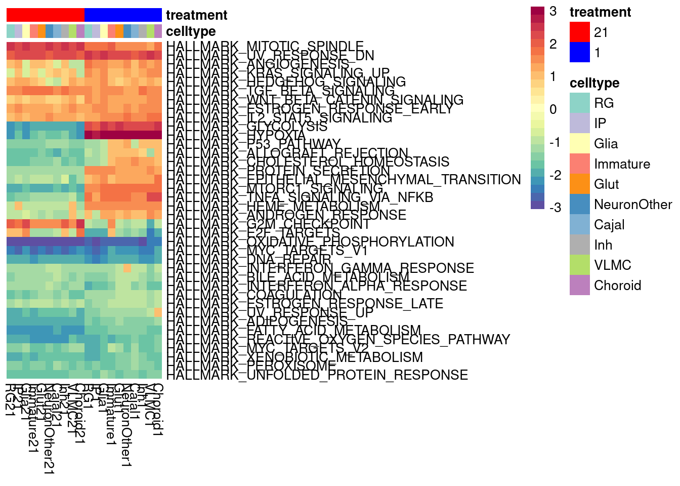
rm(combined_fgsea_all, m_posterior)

Compare DE genes to previously published findings

Here, I compare our results to the DE genes identified in Paşca et al..

m_posterior_fine <- readRDS(file="/project2/gilad/umans/oxygen_eqtl/output/mash_de/mashposterior_dataset9_fine_reharmonized_z3.RDS")

Pasca lab reported all genes with FDR<0.05 and logFC>0.58 in their supplement.

pasca24 <- read_csv(file = "/project2/gilad/umans/oxygen_eqtl/data/external/Pasca_24hr.csv")

Rows: 943 Columns: 7
── Column specification ────────────────────────────────────────────────────────
Delimiter: ","
chr (2): GeneID, GeneAnnotation
dbl (5): logFC, logCPM, F, PValue, FDR

ℹ Use `spec()` to retrieve the full column specification for this data.
ℹ Specify the column types or set `show_col_types = FALSE` to quiet this message.

pasca48 <- read_csv(file = "/project2/gilad/umans/oxygen_eqtl/data/external/Pasca_48hr.csv")

Rows: 1520 Columns: 7
── Column specification ────────────────────────────────────────────────────────
Delimiter: ","
chr (2): GeneID, GeneAnnotation
dbl (5): logFC, logCPM, F, PValue, FDR

ℹ Use `spec()` to retrieve the full column specification for this data.
ℹ Specify the column types or set `show_col_types = FALSE` to quiet this message.

length(unique(c(pasca24$GeneAnnotation, pasca48$GeneAnnotation)))

[1] 1754

This comes out to 1754 DE genes.

Now, we add these result into the mash posterior matrices in order to similarly calculate the similarity of the Pasca results to our hypoxia and hyperoxia DE genes.

m_posterior_comparison <- m_posterior_fine
m_posterior_comparison$PosteriorMean <- data.frame(m_posterior_comparison$PosteriorMean ) %>% 
  rownames_to_column(var = "GeneAnnotation") %>% 
  left_join(x=., y = (pasca24 %>% select(GeneAnnotation, Pasca124=logFC)), by=join_by("GeneAnnotation")) %>% 
  # replace_na(list(Pasca124=0)) %>%
  left_join(x=., y = (pasca48 %>% select(GeneAnnotation, Pasca148=logFC)), by=join_by("GeneAnnotation")) %>% 
  # replace_na(list(Pasca124=0)) %>%
  column_to_rownames(var = "GeneAnnotation") %>% as.matrix()

m_posterior_comparison$lfsr <- data.frame(m_posterior_comparison$lfsr ) %>% 
  rownames_to_column(var = "GeneAnnotation") %>% 
  left_join(x=., y = (pasca24 %>% select(GeneAnnotation, Pasca124=FDR)), by=join_by("GeneAnnotation")) %>% 
  # replace_na(list(Pasca124=0)) %>%
  left_join(x=., y = (pasca48 %>% select(GeneAnnotation, Pasca148=FDR)), by=join_by("GeneAnnotation")) %>% 
  # replace_na(list(Pasca124=0)) %>%
  column_to_rownames(var = "GeneAnnotation") %>% as.matrix()


shared.effect = matrix(NA,nrow = ncol(m_posterior_comparison$lfsr),ncol=ncol(m_posterior_comparison$lfsr))
colnames(shared.effect) <- rownames(shared.effect) <- colnames(m_posterior_comparison$lfsr)

for (i in 1:ncol(m_posterior_comparison$PosteriorMean)) {
  for (j in 1:ncol(m_posterior_comparison$PosteriorMean)) {
    sig.row=which(m_posterior_comparison$lfsr[,i] < 0.05)
    sig.col=which(m_posterior_comparison$lfsr[,j] < 0.05)
    size.row=which(abs(m_posterior_comparison$PosteriorMean[,i]) > 0.58)
    size.col=which(abs(m_posterior_comparison$PosteriorMean[,j]) > 0.58)
    a=intersect(intersect(sig.row,sig.col), union(size.row, size.col)) # at least one effect is significant
    # # constrain to those with at least one posterior mean logFC>0.58
    shared.effect[i,j] <- cor(m_posterior_comparison$PosteriorMean[a,i], m_posterior_comparison$PosteriorMean[a,j], use = "pairwise.complete.obs")
    
  }
}

labels <- data.frame(celltype=str_extract(rownames(shared.effect), pattern = "[:alpha:]+"),
                     treatment=str_extract(rownames(shared.effect), pattern = "[:digit:]+"))
rownames(labels) <- rownames(shared.effect)

celltypeCol <- c(manual_palette_fine, Pasca="purple")

treatmentCol <- c("red", "blue", "lightblue", "darkblue")
# names(celltypeCol) <- unique(labels$celltype)
names(treatmentCol) <- unique(labels$treatment)
annoCol <- list(celltype = celltypeCol,
                treatment = treatmentCol)

# now use pheatmap to annotate
pheatmap(shared.effect, col = viridis(50),
         border_color = NA,
         show_colnames = TRUE,
         treeheight_row = 0, treeheight_col = 0,
         annotation_row = labels,
         annotation_colors = annoCol
         )

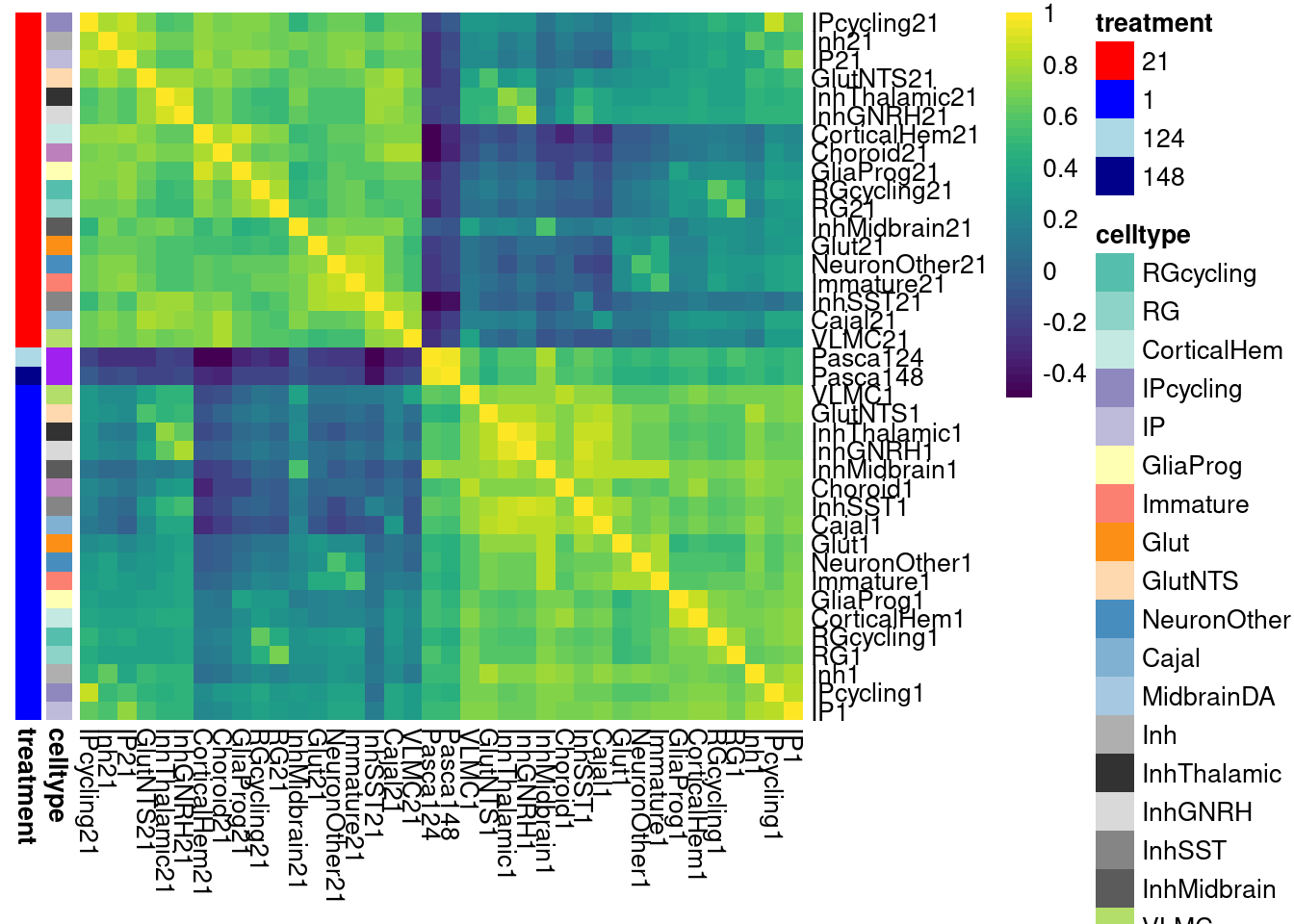
pheatmap(shared.effect[c(1:18, 37:38), c(1:18, 37:38)], col = colorRampPalette(rev(brewer.pal(11, "Spectral")))(50),
         border_color = NA,
         show_colnames = TRUE,
         treeheight_row = 0, treeheight_col = 0,
         annotation_row = labels, legend_breaks = c(-0.5, 0, 0.5, 1), drop_levels = FALSE, breaks =seq(from=-0.5, to=1, length.out=51), 
         annotation_colors = annoCol, cellwidth = 6, cellheight = 6, fontsize = 6, angle_col = 45
         )

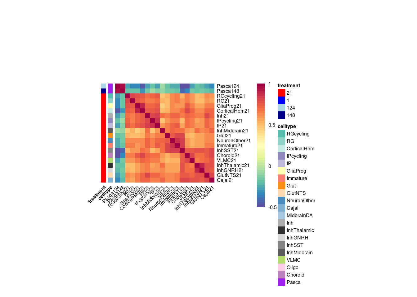
pheatmap(shared.effect[c(19:38), c(19:38)], col = colorRampPalette(rev(brewer.pal(11, "Spectral")))(50),
         border_color = NA,
         show_colnames = TRUE,
         treeheight_row = 0, treeheight_col = 0,
         annotation_row = labels, legend_breaks = c(-0.5, 0, 0.5, 1), drop_levels = FALSE, breaks =seq(from=-0.5, to=1, length.out=51), 
         annotation_colors = annoCol,  cellwidth = 6, cellheight = 6, fontsize = 6, angle_col = 45
         )

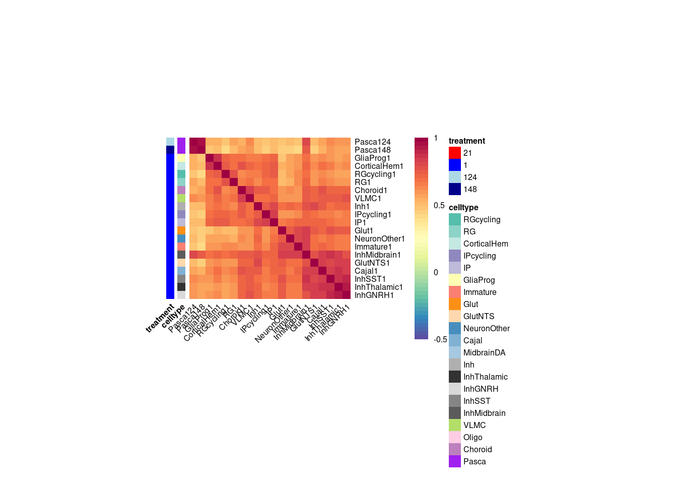
Stressed cell annotation

We used the Gruffi software tool to identify highly hypoxia- and hyperoxia-responsive cells in our dataset. Gruffi works by first clustering single-cell data very finely into “neighborhoods” of similar cells, helping to smooth some of the sparsity of single-cell measurements. Scores based on chosen gene lists are then calculated and used to set high- and low-pass filters for cell classification.

In the default Gruffi use case, “stressed” cells are identified by high expression of glycolytic and ER stress-related genes. However, in our experiment, environmental oxygen was directly modulated, meaning that responsive cells should be identifiable based on genes that change under these conditions. In our initial analyses, we confirmed that gene module scores obtained from these default gene lists were poorly correlated with the treatment condition of a given cell neighborhood, with the exception of the glycolytic (GO:0006096) gene module and hypoxia exposure. Instead, we first obtained alternative gene lists based on the estimates of DE sharing provided by mash. These gene lists were used to identify treatment-responsive cells in both the hyperoxia and hypoxia conditions separately. Note that although these gene lists are non-overlapping, it is possible for cells to be classified as hypoxia- or hyperoxia-responsive, or both, in any treatment condition, although we expect that hypoxia exposure should increase the proportion of hypoxia-responsive cells and decrease hyperoxia-responsive cells, and vice-versa.

m_posterior <- readRDS(file="/project2/gilad/umans/oxygen_eqtl/output/mash_de/mashposterior_dataset9_fine_reharmonized_z3.RDS")

m_posterior_hypoxia<- list()
m_posterior_hypoxia$lfsr <- m_posterior$lfsr[,c("RGcycling1", "InhThalamic1", "InhSST1",  "InhGNRH1", "IPcycling1", "GlutNTS1", "GliaProg1", "CorticalHem1", "Inh1", "Cajal1", "Choroid1", "VLMC1", "NeuronOther1", "Immature1", "IP1", "RG1", "Glut1")]
m_posterior_hypoxia$PosteriorMean <- m_posterior$PosteriorMean[,c("RGcycling1", "InhThalamic1", "InhSST1",  "InhGNRH1", "IPcycling1", "GlutNTS1", "GliaProg1", "CorticalHem1", "Inh1", "Cajal1", "Choroid1", "VLMC1", "NeuronOther1", "Immature1", "IP1", "RG1", "Glut1")]

# start with genes that are significantly DE in all tested cell types 
gene.filter <- apply(m_posterior_hypoxia$lfsr, MARGIN = 1, function(i)sum(i>0.05))
shared.genes <- names(gene.filter)[which(gene.filter==0)]

filtered.shared.genes.hypoxia <- shared.genes[apply(m_posterior_hypoxia$PosteriorMean[shared.genes,], MARGIN = 1, FUN = function(x){all(abs(x)/median(abs(x))<5 & sign(x)>0) & mean(x)>1 })]

filtered.shared.genes.hypoxia

 [1] "BNIP3"       "IGFBP2"      "PGAM1"       "BNIP3L"      "FAM162A"    
 [6] "TPI1"        "PGK1"        "P4HA1"       "ENO1"        "LDHA"       
[11] "MIR210HG"    "ALDOA"       "AC097534.2"  "MTFP1"       "AK4"        
[16] "SLC2A1"      "VEGFA"       "PDK1"        "RCOR2"       "ANKRD37"    
[21] "PLOD2"       "HK2"         "TNIP1"       "DDIT4"       "AC107021.1" 
[26] "INSIG2"      "WSB1"        "NRN1"        "PPFIA4"      "EGLN1"      
[31] "RAPGEF4"     "FAM210A"     "P4HA2"       "CXCR4"       "GOLGA8A"    
[36] "ENO2"        "SNHG19"      "GPI"         "HLA-B"       "MT3"        
[41] "ADAMTS20"    "PFKP"        "PFKFB3"      "HILPDA"      "KDM3A"      
[46] "RLF"         "KDM7A"       "AC087280.2"  "HK1"         "PDK3"       
[51] "LINC02649"   "FUT11"       "NIM1K"       "COL11A1"     "AL357153.2" 
[56] "KDM4C"       "UACA"        "SLC16A1"     "USP28"       "SLC8A3"     
[61] "RASGRF1"     "NRIP3"       "PRMT8"       "NDRG1"       "PCAT6"      
[66] "RAPGEF4-AS1"

m_posterior_hyperoxia<- list()
m_posterior_hyperoxia$lfsr <- m_posterior$lfsr[,c("RGcycling21", "InhThalamic21", "InhSST21",  "InhGNRH21", "IPcycling21", "GlutNTS21", "GliaProg21", "CorticalHem21", "Inh21", "Cajal21", "Choroid21", "VLMC21", "NeuronOther21", "Immature21", "IP21", "RG21", "Glut21")]

m_posterior_hyperoxia$PosteriorMean <- m_posterior$PosteriorMean[,c("RGcycling21", "InhThalamic21", "InhSST21", "InhGNRH21", "IPcycling21", "GlutNTS21", "GliaProg21", "CorticalHem21", "Inh21", "Cajal21", "Choroid21", "VLMC21", "NeuronOther21", "Immature21", "IP21", "RG21", "Glut21")]


gene.filter <- apply(m_posterior_hyperoxia$lfsr, MARGIN = 1, function(i)sum(i>0.05))
shared.genes <- names(gene.filter)[which(gene.filter==0)]

filtered.shared.genes.hyperoxia <- shared.genes[apply(m_posterior_hyperoxia$PosteriorMean[shared.genes,], MARGIN = 1, FUN = function(x){all(abs(x)/median(abs(x))<5 & sign(x)>0) & mean(x)>0.6 })]

filtered.shared.genes.hyperoxia

[1] "RPS20"     "RBM3"      "NUDT3"     "USP13"     "GALNT17"   "LINC01619"
[7] "SLC7A11"  

Note that these are distinct gene sets.

length(intersect(filtered.shared.genes.hyperoxia, filtered.shared.genes.hypoxia))

[1] 0

These gene sets were then used as input for Gruffi, following their standard workflow outlined on the software’s Github page.

library(gruffi)

harmony.batchandindividual.sct <- Seurat.utils::SetupReductionsNtoKdimensions(obj = harmony.batchandindividual.sct, nPCs = 50, dimensions=3:2, reduction="umap")
harmony.batchandindividual.sct <- AutoFindGranuleResolution(obj = harmony.batchandindividual.sct, assay = "SCT")
granule.res.4.gruffi <- harmony.batchandindividual.sct@misc$gruffi$'optimal.granule.res'
harmony.batchandindividual.sct <- ReassignSmallClusters(harmony.batchandindividual.sct, ident = granule.res.4.gruffi) 
granule.res.4.gruffi <- paste0(granule.res.4.gruffi, '.reassigned')

Score the default Gruffi GO terms as well as our custom gene lists:

go1 <- "GO:0006096" # Glycolysis
go2 <- "GO:0034976" # ER-stress
go3 <- "GO:0042063" # Gliogenesis, negative filtering
# Glycolytic process    GO:0006096
harmony.batchandindividual.sct <- AssignGranuleAverageScoresFromGOterm(obj = harmony.batchandindividual.sct, GO_term = go1, save.UMAP = TRUE, new_GO_term_computation = T, clustering = granule.res.4.gruffi, plot.each.gene = F)

# ER stress     GO:0034976
harmony.batchandindividual.sct <- AssignGranuleAverageScoresFromGOterm(obj = harmony.batchandindividual.sct, GO_term = go2, save.UMAP = TRUE, new_GO_term_computation = T, clustering = granule.res.4.gruffi, plot.each.gene = F)

# Gliogenesis       GO:0042063
harmony.batchandindividual.sct <- AssignGranuleAverageScoresFromGOterm(obj = harmony.batchandindividual.sct, GO_term = go3, save.UMAP = TRUE, new_GO_term_computation = T, clustering = granule.res.4.gruffi, plot.each.gene = F)

Score the custom gene lists:

harmony.batchandindividual.sct <- AddModuleScore(harmony.batchandindividual.sct, features = list(filtered.shared.genes.hypoxia), assay = "RNA", name = "mash_hypoxia")

harmony.batchandindividual.sct <- CustomScoreEvaluation(obj = harmony.batchandindividual.sct, custom.score.name = "mash_hypoxia1", clustering = "SCT_snn_res.105.reassigned")

# due to a bug in this version of Gruffi, custom scores are stored as factors rather than numeric values, so that needs to be converted before further calculations
harmony.batchandindividual.sct$SCT_snn_res.105.reassigned_cl.av_mash_hypoxia1 <- as.numeric(levels(harmony.batchandindividual.sct$SCT_snn_res.105.reassigned_cl.av_mash_hypoxia1))[harmony.batchandindividual.sct$SCT_snn_res.105.reassigned_cl.av_mash_hypoxia1]

harmony.batchandindividual.sct <- AddModuleScore(harmony.batchandindividual.sct, features = list(filtered.shared.genes.hyperoxia), assay = "RNA", name = "mash_hyperoxia")

harmony.batchandindividual.sct <- CustomScoreEvaluation(obj = harmony.batchandindividual.sct, custom.score.name = "mash_hyperoxia1", clustering = "SCT_snn_res.105.reassigned")

# due to a bug in this version of Gruffi, custom scores are stored as factors rather than numeric values, so that needs to be converted before further calculations
harmony.batchandindividual.sct$SCT_snn_res.105.reassigned_cl.av_mash_hyperoxia1 <- as.numeric(levels(harmony.batchandindividual.sct$SCT_snn_res.105.reassigned_cl.av_mash_hyperoxia1))[harmony.batchandindividual.sct$SCT_snn_res.105.reassigned_cl.av_mash_hyperoxia1]

Now use Gruffi’s interactive tool to check the thresholded scores. Here, I use only the custom-calculated scores and the default negative selection score, and allow the thresholds to be chosen automatically.

i1 <- "SCT_snn_res.105.reassigned_cl.av_mash_hypoxia1"
(i3 <- Stringendo::kppu(granule.res.4.gruffi, 'cl.av', "GO.0042063"))

# Call Shiny app
harmony.batchandindividual.sct <- FindThresholdsShiny(obj = harmony.batchandindividual.sct,
                                stress.ident1 = i1,
                                stress.ident2 = i1,
                                notstress.ident3 = i3)
# Mash score auto set at 3.421, gliogenesis score auto set at 3.191

meta_export <- harmony.batchandindividual.sct@meta.data
saveRDS(meta_export, file = "post_gruffi_metadata_hypoxia_mash_reharmonized_remashed.RDS")

i1 <- "SCT_snn_res.105.reassigned_cl.av_mash_hyperoxia1"

# Call Shiny app
harmony.batchandindividual.sct <- FindThresholdsShiny(obj = harmony.batchandindividual.sct,
                                stress.ident1 = i1,
                                stress.ident2 = i1,
                                notstress.ident3 = i3)
# mash score auto set to 4.832, gliogenesis score auto set to 3.191

meta_export_hyperox <- harmony.batchandindividual.sct@meta.data
saveRDS(meta_export_hyperox, file = "post_gruffi_metadata_hyperox_mash_reharmonized_remashed.RDS")

I also do the same for the default Gruffi gene sets:

(i1 <- Stringendo::kppu(granule.res.4.gruffi, 'cl.av', "GO.0006096"))
(i2 <- Stringendo::kppu(granule.res.4.gruffi, 'cl.av', "GO.0034976"))
(i3 <- Stringendo::kppu(granule.res.4.gruffi, 'cl.av', "GO.0042063"))

# Call Shiny app
harmony.batchandindividual.sct <- FindThresholdsShiny(obj = harmony.batchandindividual.sct,
                                stress.ident1 = i1,
                                stress.ident2 = i2,
                                notstress.ident3 = i3)

# auto thresholds are 2.488 for GO.0006096, 1.429 for GO.0034976, and 3.191 for GO.0042063
meta_export_default <- harmony.batchandindividual.sct@meta.data
saveRDS(meta_export_default, file = "post_gruffi_metadata_default_mash_reharmonized.RDS")

Next, attach the hypoxia and hyperoxia response annotations from Gruffi to the working Seurat object and classify cells as responsive/unresponsive. Now do the same with the mash scores

hypoxia_stressed_mash <- readRDS(file = "/project2/gilad/umans/oxygen_eqtl/output/post_gruffi_metadata_hypoxia_mash_reharmonized_remashed.RDS") %>% select(hypoxia_stressed_mash = `is.Stressed`)
hyperoxia_stressed_mash <- readRDS(file = "/project2/gilad/umans/oxygen_eqtl/output/post_gruffi_metadata_hyperox_mash_reharmonized_remashed.RDS") %>% select(hyperoxia_stressed_mash= `is.Stressed`)

harmony.batchandindividual.sct <- AddMetaData(harmony.batchandindividual.sct, metadata = hypoxia_stressed_mash)
harmony.batchandindividual.sct <- AddMetaData(harmony.batchandindividual.sct, metadata = hyperoxia_stressed_mash)
# and, add a combined column called "gruffi_label" that incorporates both hypoxia and hyperoxia stress scores
harmony.batchandindividual.sct$gruffi_label_mash <- harmony.batchandindividual.sct@meta.data %>% select(hypoxia_stressed_mash, hyperoxia_stressed_mash) %>% mutate(hypoxia = 2* hypoxia_stressed_mash) %>% mutate(stressed = hyperoxia_stressed_mash + hypoxia)  %>% mutate(stressed_label = case_match(stressed, 0 ~ "unstressed", 1 ~ "hyperoxia_stressed", 2 ~ "hypoxia_stressed", 3 ~ "double_stressed")) %>% select(stressed_label)

For the default Gruffi gene sets, I will do this only for the hypoxia condition, as we previously determined that the scores are largely unresponsive to hyperoxic treatment:

hypoxia_stressed <- readRDS(file = "/project2/gilad/umans/oxygen_eqtl/output/post_gruffi_metadata_default_mash_reharmonized.RDS") %>% select(hypoxia_stressed = `is.Stressed`)

harmony.batchandindividual.sct <- AddMetaData(harmony.batchandindividual.sct, metadata = hypoxia_stressed)
# and, add a combined column called "gruffi_label" that incorporates both hypoxia and hyperoxia stress scores
harmony.batchandindividual.sct$gruffi_label <- harmony.batchandindividual.sct@meta.data %>% 
  select(hypoxia_stressed) %>%
  mutate(stressed = 1* hypoxia_stressed)  %>% 
  mutate(stressed_label = case_match(stressed, 0 ~ "unstressed", 1 ~ "hypoxia_stressed")) %>%
  select(stressed_label)

Now, for both the fine and coarse clustering, calculate the fractional change in the responsive cell proportion across treatment conditions.

First, in the coarse classification:

stressed_table <- as.data.frame(table(harmony.batchandindividual.sct$gruffi_label_mash, harmony.batchandindividual.sct$combined.annotation.coarse.harmony, harmony.batchandindividual.sct$treatment)) %>%
  mutate(Freq = Freq+1) %>% #add pseudocount of one cell to avoid a divide by potential zero problem
  group_by(Var3, Var2) %>%
  mutate(totals=sum(Freq)) %>% 
  ungroup() %>% 
  mutate(fraction=round(Freq/totals, digits=3))

stressed_table %>% dplyr::select(Var1, Var2, Var3, fraction) %>% 
  pivot_wider(names_from = Var3, values_from = fraction) %>% 
  mutate(control10 =  na_if(x = control10, y = 0)) %>% mutate(change1_10=(stim1pct-control10)/control10) %>%  
  replace_na(list(change1_10=0)) %>% 
  # filter(Var1 != "double_stressed")  %>%
  # filter(Var1 != "unstressed") %>% 
  # filter(Var1 != "hyperoxia_stressed") %>% 
  ggplot(aes(x=reorder(Var2, -change1_10), y=change1_10, color=Var1)) + 
  geom_point(size=2) + 
  coord_flip() + 
  ylab("Gruffi (mash) stress fraction change (control vs 1%)") + 
  xlab("Cell type") +  
  scale_color_manual(values = c("unstressed"= "#abd9e9", "hypoxia_stressed" = "#d7191c", "hyperoxia_stressed"= "#fdae61", "double_stressed" = "purple"),  name="Stress classification") + 
  theme_light()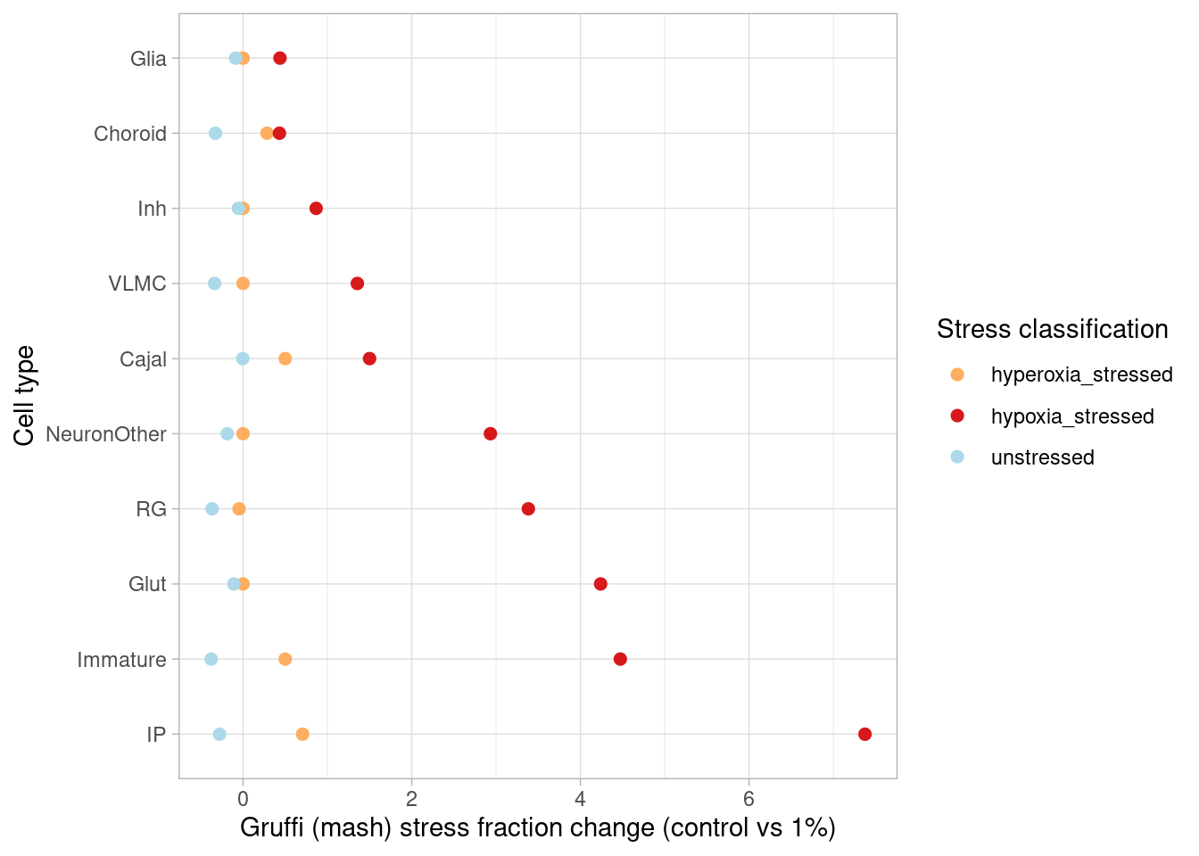

Past versions of unnamed-chunk-74-1.png

Version	Author	Date
e2547f5	Ben Umans	2025-02-24

stressed_table %>% dplyr::select(Var1, Var2, Var3, fraction) %>% 
  pivot_wider(names_from = Var3, values_from = fraction) %>% 
  mutate(control10 =  na_if(x = control10, y = 0)) %>% 
  mutate(change21_10=(stim21pct-control10)/control10) %>%  
  replace_na(list(change21_10=0)) %>% 
  # filter(Var1 != "double_stressed")  %>%
  # filter(Var1 != "unstressed") %>% 
  ggplot(aes(x=reorder(Var2, -change21_10), y=change21_10, color=Var1)) + 
  geom_point(size=2) + 
  coord_flip() + 
  ylab("Gruffi (mash) stress fraction change (control vs 21%)") + 
  xlab("Cell type")+  
  scale_color_manual(values = c("unstressed"= "#abd9e9", "hypoxia_stressed" = "#d7191c", "hyperoxia_stressed"= "#fdae61", "double_stressed" = "purple"), name="Stress classification") +
  theme_light()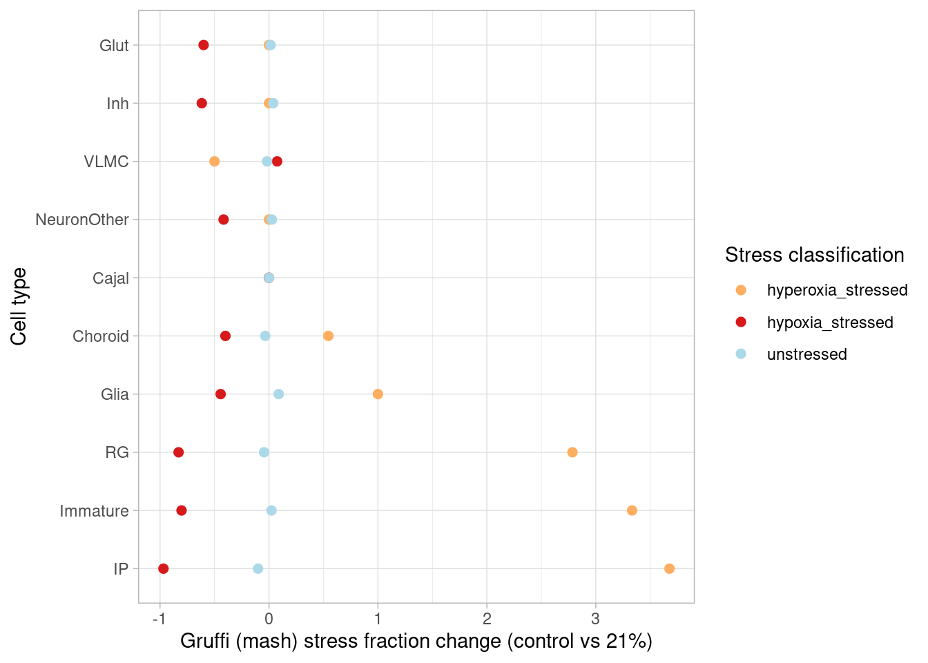

Past versions of unnamed-chunk-74-2.png

Version	Author	Date
e2547f5	Ben Umans	2025-02-24

Now using the fine classification:

stressed_table <- as.data.frame(table(harmony.batchandindividual.sct$gruffi_label_mash, harmony.batchandindividual.sct$combined.annotation.fine.harmony, harmony.batchandindividual.sct$treatment)) %>%
  mutate(Freq = Freq+1) %>%
  group_by(Var3, Var2) %>% 
  mutate(totals=sum(Freq)) %>%
  ungroup() %>%
  mutate(fraction=round(Freq/totals, digits=3))

stressed_table %>% dplyr::select(Var1, Var2, Var3, fraction) %>% 
  pivot_wider(names_from = Var3, values_from = fraction) %>% 
  mutate(control10 =  na_if(x = control10, y = 0)) %>% 
  mutate(change1_10=(stim1pct-control10)/control10) %>%  
  replace_na(list(change1_10=0)) %>% 
  # filter(Var1 != "double_stressed")  %>%
  # filter(Var1 != "unstressed") %>% 
  ggplot(aes(x=reorder(Var2, -change1_10), y=change1_10, color=Var1)) +
  geom_point(size=2) + 
  coord_flip() + 
  ylab("Gruffi (mash) stress fraction change (control vs 1%)") + 
  xlab("Cell type") +  
  scale_color_manual(values = c("unstressed"= "#abd9e9", "hypoxia_stressed" = "#d7191c", "hyperoxia_stressed"= "#fdae61", "double_stressed" = "purple"), name="Stress classification") + 
  theme_light()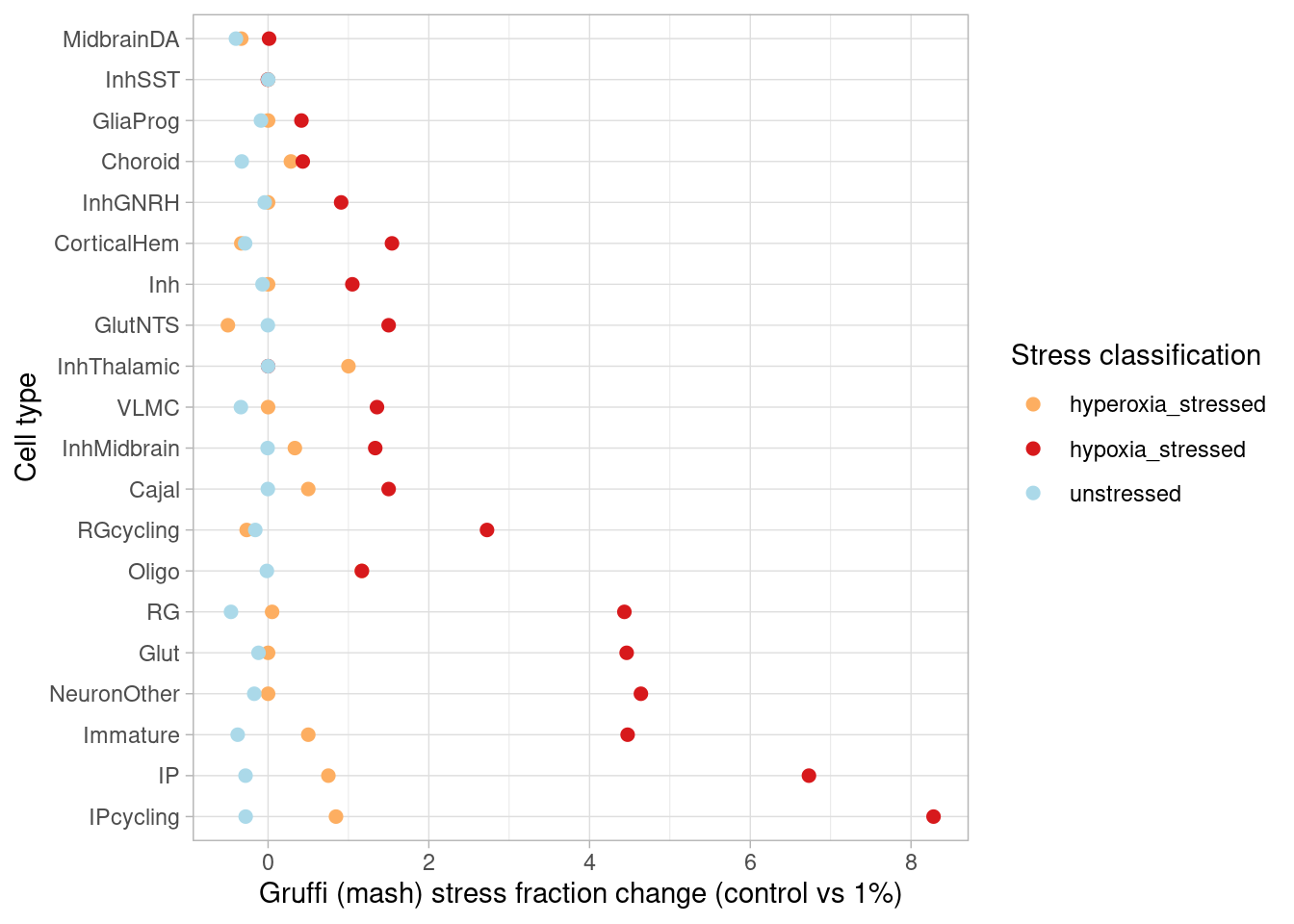

Past versions of unnamed-chunk-75-1.png

Version	Author	Date
e2547f5	Ben Umans	2025-02-24

stressed_table %>% dplyr::select(Var1, Var2, Var3, fraction) %>% 
  pivot_wider(names_from = Var3, values_from = fraction) %>% 
  mutate(control10 =  na_if(x = control10, y = 0)) %>%
  mutate(change21_10=(stim21pct-control10)/control10) %>%  
  replace_na(list(change21_10=0)) %>% 
  # filter(Var1 != "double_stressed")  %>%
  # filter(Var1 != "unstressed") %>% 
  ggplot(aes(x=reorder(Var2, -change21_10), y=change21_10, color=Var1)) + 
  geom_point(size=2) + 
  coord_flip() + 
  ylab("Gruffi (mash) stress fraction change (control vs 21%)") +
  xlab("Cell type") +
  scale_color_manual(values = c("unstressed"= "#abd9e9", "hypoxia_stressed" = "#d7191c", "hyperoxia_stressed"= "#fdae61", "double_stressed" = "purple"), name="Stress classification") +
  theme_light()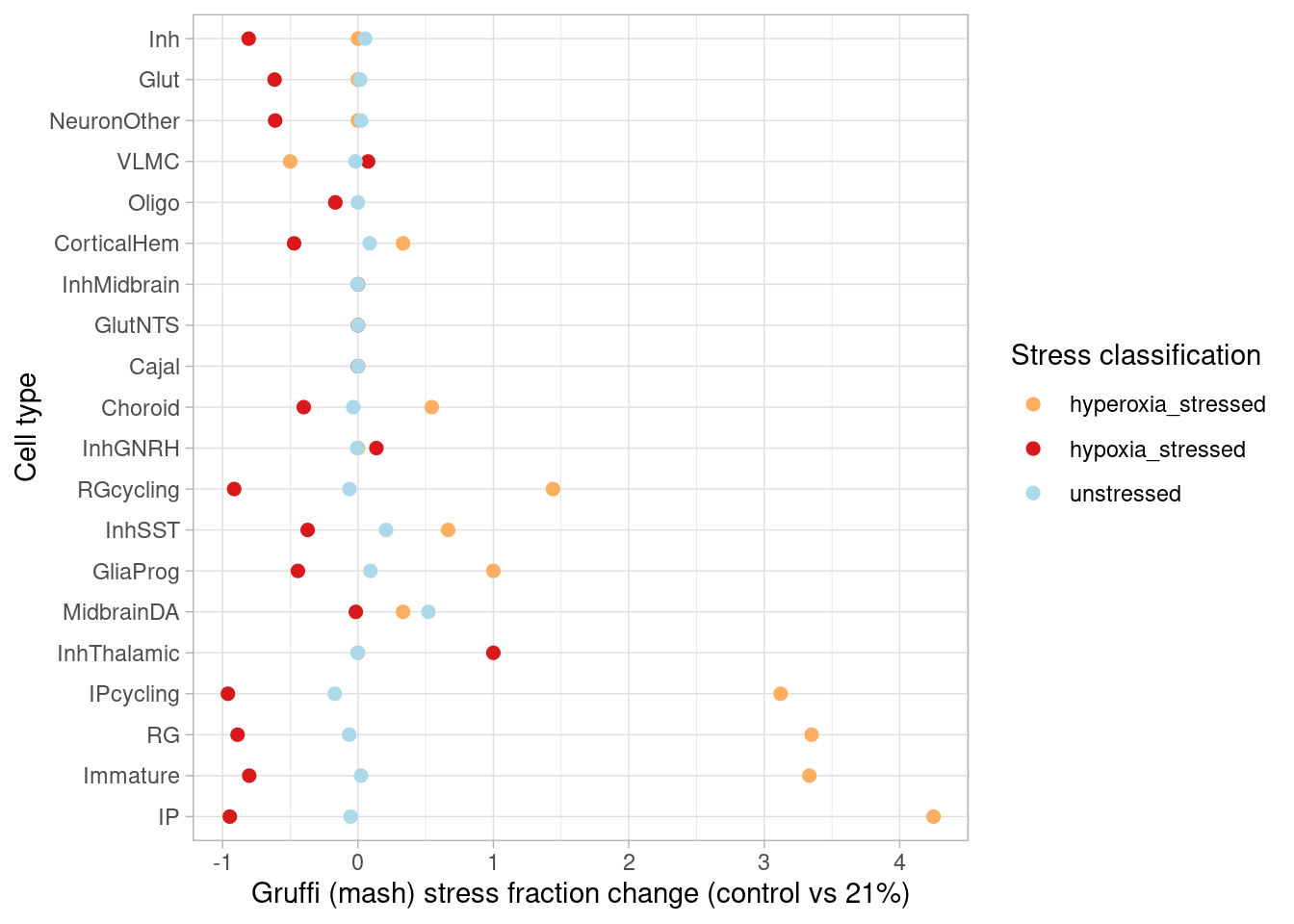

Past versions of unnamed-chunk-75-2.png

Version	Author	Date
e2547f5	Ben Umans	2025-02-24

Plot the default Gruffi scores:

stressed_table <- as.data.frame(table(harmony.batchandindividual.sct$gruffi_label, harmony.batchandindividual.sct$combined.annotation.coarse.harmony, harmony.batchandindividual.sct$treatment)) %>%
  mutate(Freq = Freq+1) %>% 
  group_by(Var3, Var2) %>% 
  mutate(totals=sum(Freq)) %>% 
  ungroup() %>% mutate(fraction=round(Freq/totals, digits=3))

stressed_table %>% dplyr::select(Var1, Var2, Var3, fraction) %>% 
  pivot_wider(names_from = Var3, values_from = fraction) %>% 
  mutate(control10 =  na_if(x = control10, y = 0)) %>% 
  mutate(change1_10=(stim1pct-control10)/control10) %>%  
  replace_na(list(change1_10=0)) %>% 
  filter(Var1 != "unstressed") %>%
  ggplot(aes(x=reorder(Var2, -change1_10), y=change1_10, color=Var1)) + 
  geom_point(size=2) + 
  coord_flip() + 
  ylab("Gruffi (default) stress fraction change (control vs 1%)") + 
  xlab("Cell type") + 
  scale_color_manual(values = c("unstressed"= "#abd9e9", "hypoxia_stressed" = "#d7191c"), name="Stress classification") +
  theme_light()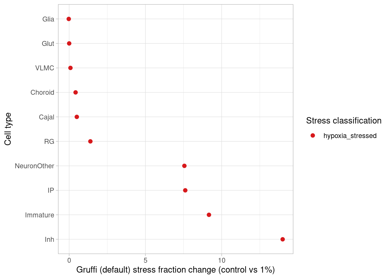

Past versions of unnamed-chunk-76-1.png

Version	Author	Date
e2547f5	Ben Umans	2025-02-24

stressed_table <- as.data.frame(table(harmony.batchandindividual.sct$gruffi_label, harmony.batchandindividual.sct$combined.annotation.fine.harmony, harmony.batchandindividual.sct$treatment)) %>%
  group_by(Var3, Var2) %>%
  mutate(totals=sum(Freq)) %>%
  ungroup() %>% 
  mutate(fraction=round(Freq/totals, digits=3))

stressed_table %>% 
  select(Var1, Var2, Var3, fraction) %>%
  pivot_wider(names_from = Var3, values_from = fraction) %>%
  mutate(control10 =  na_if(control10, 0)) %>%
  mutate(change1_10=(stim1pct-control10)/control10) %>%
  replace_na(list(change1_10=0)) %>%
  filter(Var1 != "unstressed") %>%
  ggplot(aes(x=reorder(Var2, -change1_10), y=change1_10, color=Var1)) + 
  geom_point() + 
  coord_flip() + 
  ylab("Gruffi (default) stress fraction change (control vs 1%)") + 
  xlab("Cell type")+ 
  scale_color_manual(values = c("unstressed"= "#abd9e9", "hypoxia_stressed" = "#d7191c"), name="Stress classification") +
  theme_light()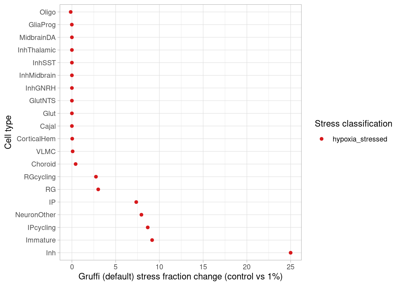

Look at the individual variability in hypoxia scores by individual in the coarse groupings:

stressed_table <- as.data.frame(table(harmony.batchandindividual.sct$gruffi_label_mash, harmony.batchandindividual.sct$combined.annotation.coarse.harmony, harmony.batchandindividual.sct$treatment, harmony.batchandindividual.sct$vireo.individual)) %>% 
  mutate(Freq = Freq+1) %>%
  group_by(Var3, Var2, Var4) %>% 
  mutate(totals=sum(Freq)) %>% 
  ungroup() %>%
  mutate(fraction=round(Freq/totals, digits=3))

stressed_table %>% 
  dplyr::select(Var1, Var2, Var3, Var4, fraction) %>%
  pivot_wider(names_from = Var3, values_from = fraction) %>%
  mutate(control10 =  na_if(control10, 0)) %>%
  mutate(change1_10=(stim1pct-control10)/control10) %>%
  replace_na(list(change1_10=0)) %>%
  filter(Var1 != "double_stressed")  %>%
  filter(Var1 != "unstressed") %>%
  filter(Var1 != "hyperoxia_stressed") %>%
  ggplot(aes(x=reorder(Var2, -change1_10), y=change1_10, color=Var1)) +
  geom_point() + 
  coord_flip() + 
  ylab("Gruffi (mash) stress fraction change (control vs 1%)") +
  xlab("Cell type") +
  scale_color_manual(values = c("unstressed"= "#abd9e9", "hypoxia_stressed" = "#d7191c", "hyperoxia_stressed"= "#fdae61", "double_stressed" = "purple")) + 
  theme_light() + scale_y_break(c(80, 120),  ticklabels = c(124))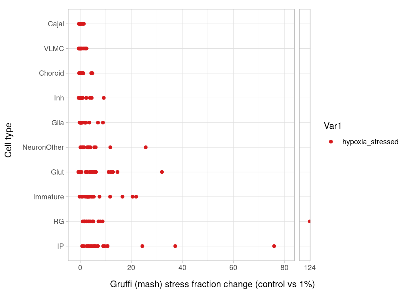

Past versions of unnamed-chunk-77-1.png

Version	Author	Date
e2547f5	Ben Umans	2025-02-24

  # scale_y_break(c(60, 185),  ticklabels = c(186))


stressed_table %>% 
  dplyr::select(Var1, Var2, Var3, Var4, fraction) %>%
  pivot_wider(names_from = Var3, values_from = fraction) %>%
  mutate(control10 =  na_if(control10, 0)) %>%
  mutate(change21_10=(stim21pct-control10)/control10) %>%
  replace_na(list(change1_10=0)) %>%
  filter(Var1 != "double_stressed")  %>%
  filter(Var1 != "unstressed") %>%
  filter(Var1 != "hypoxia_stressed") %>%
  ggplot(aes(x=reorder(Var2, -change21_10), y=change21_10, color=Var1)) +
  geom_point() + 
  coord_flip() + 
  ylab("Gruffi (mash) stress fraction change (control vs 21%)") +
  xlab("Cell type") +
  scale_color_manual(values = c("unstressed"= "#abd9e9", "hypoxia_stressed" = "#d7191c", "hyperoxia_stressed"= "#fdae61", "double_stressed" = "purple")) + 
  theme_light()

Warning: Removed 1 rows containing missing values (`geom_point()`).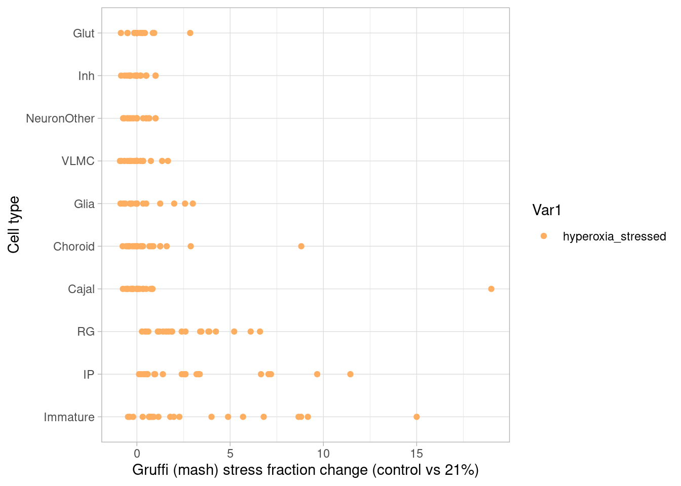

Past versions of unnamed-chunk-77-2.png

Version	Author	Date
e2547f5	Ben Umans	2025-02-24

Cell type markers in responsive cells

Treatment-responsive cells do not represent distinct cell types. As an illustration of this, I looked at a few markers of radial glia, immature neurons, intermediate progenitors, and dividing cells (comprised of radial glia and intermediate progenitors) in order to confirm that their distinct cell type markers are not lost after treatment.

colors=c("unstressed"= "#abd9e9", "hypoxia_stressed" = "#d7191c", "hyperoxia_stressed"= "#fdae61", "double_stressed" = "purple")
ip_subset <- subset(harmony.batchandindividual.sct, subset = combined.annotation.coarse.harmony=="IP")
ip_subset$gruffi_label_mash <- factor(ip_subset$gruffi_label_mash, levels = c("unstressed", "hypoxia_stressed", "hyperoxia_stressed", "double_stressed"))

VlnPlot(ip_subset, features = "EOMES", group.by = "gruffi_label_mash", y.max=3, cols=colors) + NoLegend()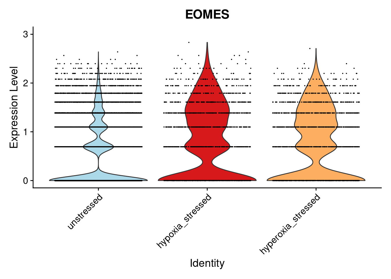

Past versions of unnamed-chunk-78-1.png

Version	Author	Date
e2547f5	Ben Umans	2025-02-24

For radial glia:

rg_subset <- subset(harmony.batchandindividual.sct, subset = combined.annotation.coarse.harmony=="RG" & gruffi_label != "double_stressed"  & gruffi_label_mash != "double_stressed")

rg_subset$gruffi_label_mash <- factor(rg_subset$gruffi_label_mash, levels = c("unstressed", "hypoxia_stressed", "hyperoxia_stressed", "double_stressed"))

VlnPlot(rg_subset, features = "LIFR", group.by = "gruffi_label_mash", y.max=3, cols=colors) + NoLegend()

Warning: Removed 1 rows containing non-finite values (`stat_ydensity()`).

Warning: Removed 1 rows containing missing values (`geom_point()`).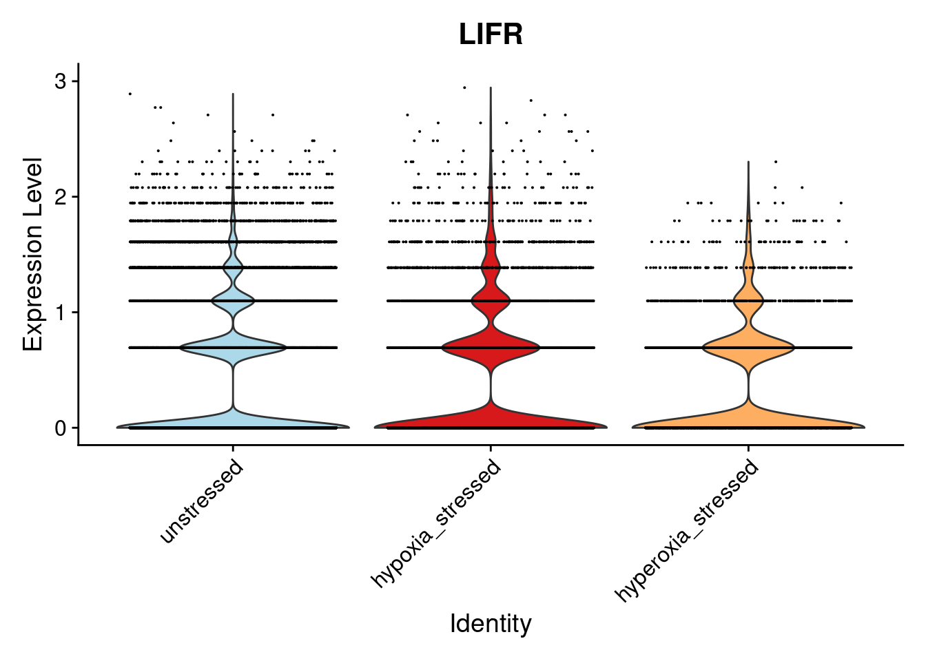

Past versions of unnamed-chunk-79-1.png

Version	Author	Date
e2547f5	Ben Umans	2025-02-24

VlnPlot(rg_subset, features = "SLC1A3", group.by = "gruffi_label_mash", cols=colors) + NoLegend()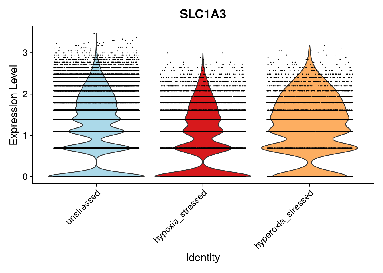

Past versions of unnamed-chunk-79-2.png

Version	Author	Date
e2547f5	Ben Umans	2025-02-24

VlnPlot(rg_subset, features = "PDGFD", group.by = "gruffi_label_mash", y.max=3, cols=colors) + NoLegend()

Warning: Removed 1 rows containing non-finite values (`stat_ydensity()`).
Removed 1 rows containing missing values (`geom_point()`).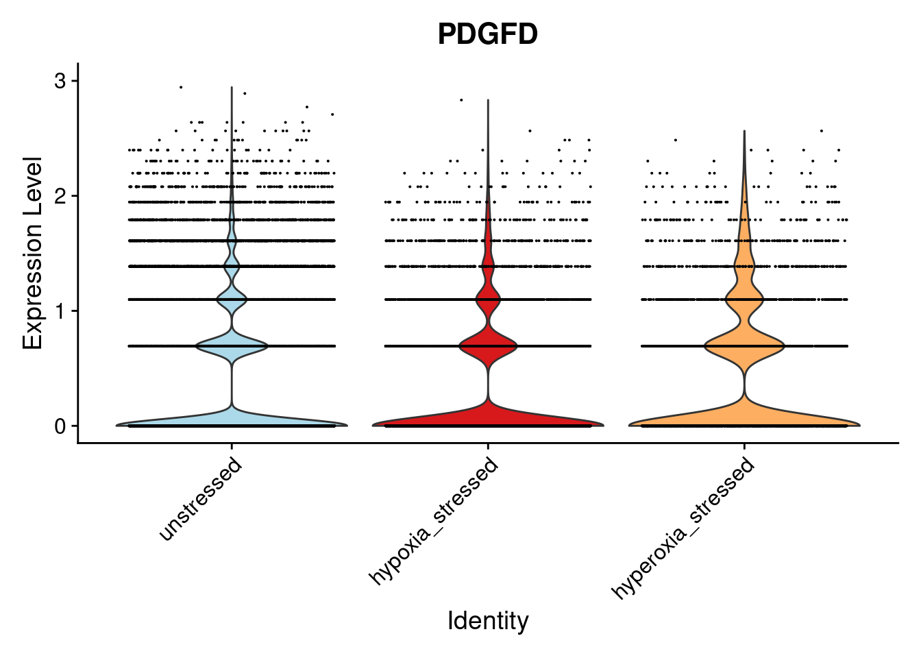

Past versions of unnamed-chunk-79-3.png

Version	Author	Date
e2547f5	Ben Umans	2025-02-24

VlnPlot(rg_subset, features = "GLI3", group.by = "gruffi_label_mash", y.max=3, cols=colors) + NoLegend()

Warning: Removed 1 rows containing non-finite values (`stat_ydensity()`).
Removed 1 rows containing missing values (`geom_point()`).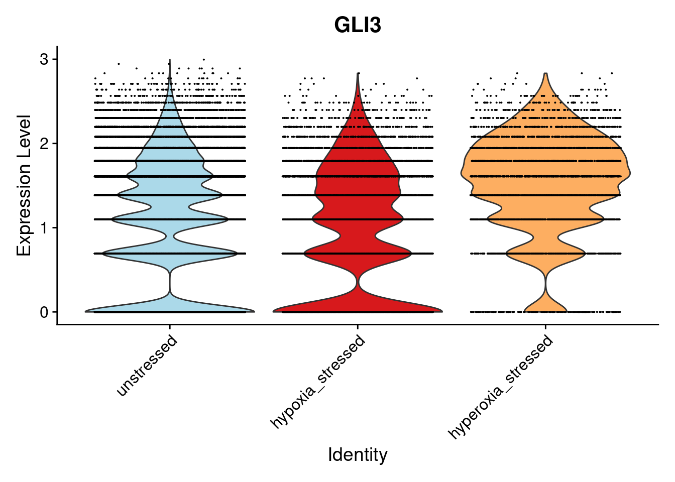

VlnPlot(rg_subset, features = "PAX6", group.by = "gruffi_label_mash", y.max=3, cols=colors) + NoLegend()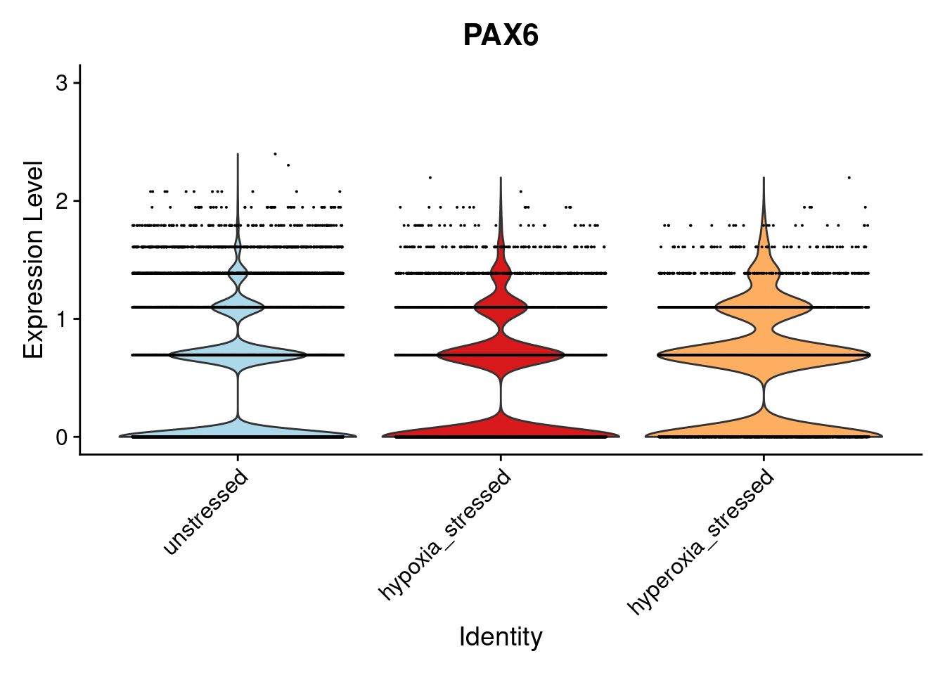

VlnPlot(rg_subset, features = "SOX2", group.by = "gruffi_label_mash", y.max=3, cols=colors) + NoLegend()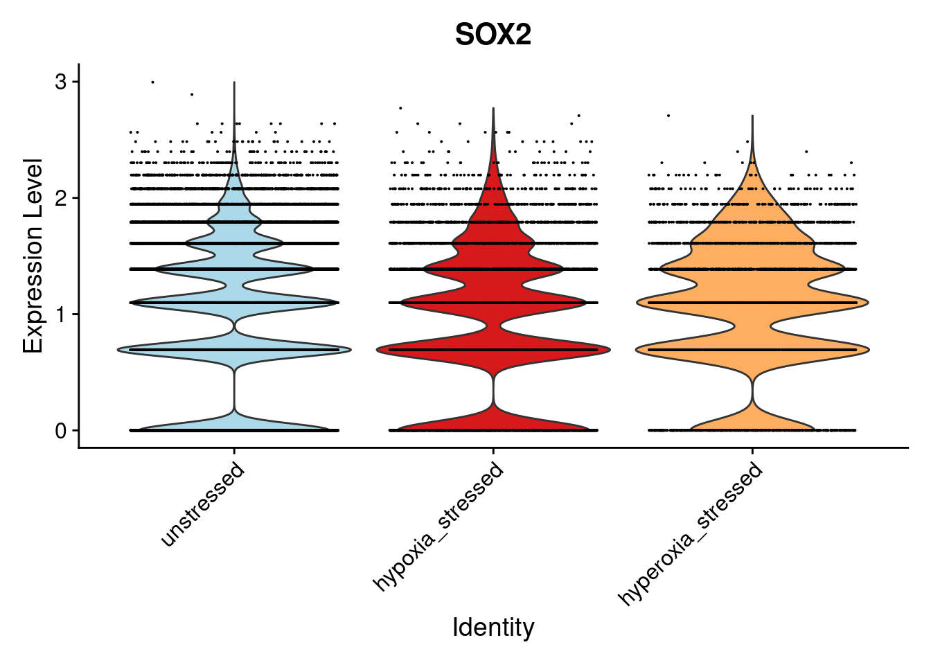

For dividing cells:

cycling_subset <- subset(harmony.batchandindividual.sct, subset = combined.annotation.fine.harmony=="RGcycling" & gruffi_label != "double_stressed"  & gruffi_label_mash != "double_stressed")
cycling_subset$gruffi_label_mash <- factor(cycling_subset$gruffi_label_mash, levels = c("unstressed", "hypoxia_stressed", "hyperoxia_stressed", "double_stressed"))

VlnPlot(cycling_subset, features = "TOP2A", group.by = "gruffi_label_mash", y.max=4, cols=colors) + NoLegend()

Warning: Removed 1 rows containing non-finite values (`stat_ydensity()`).

Warning: Removed 1 rows containing missing values (`geom_point()`).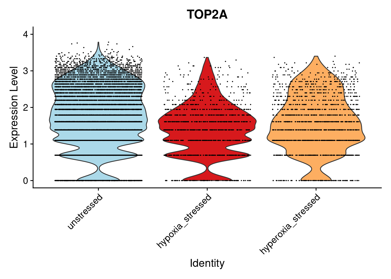

VlnPlot(cycling_subset, features = "CENPF", group.by = "gruffi_label_mash", y.max=4, cols=colors) + NoLegend()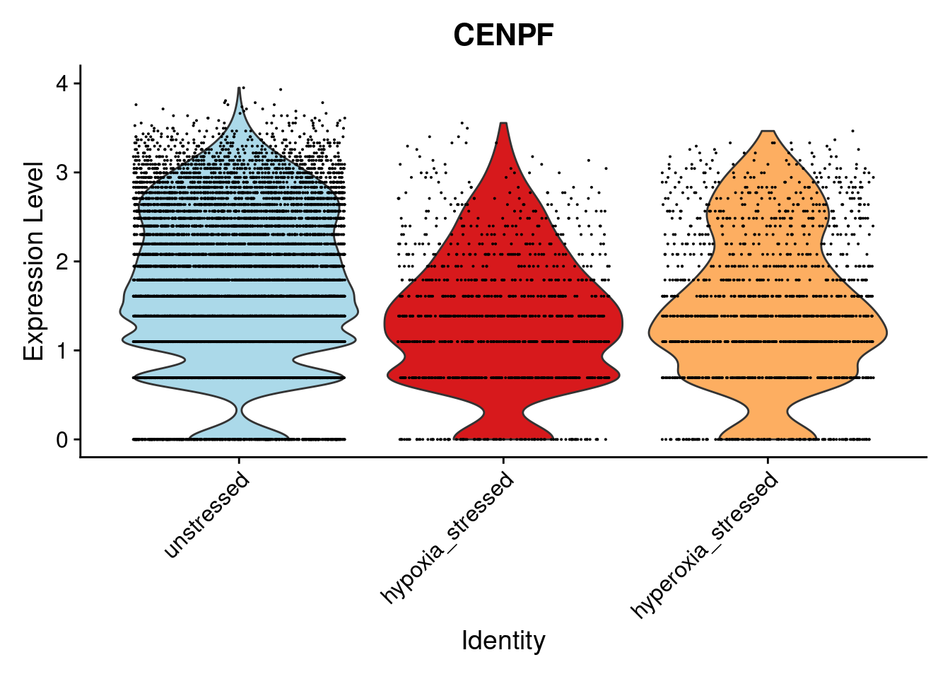

VlnPlot(cycling_subset, features = "MKI67", group.by = "gruffi_label_mash", y.max=3, cols=colors) + NoLegend()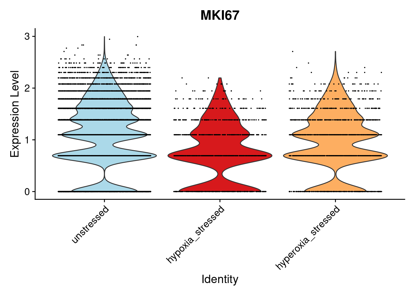

Finally, immature neurons:

immature_subset <- subset(harmony.batchandindividual.sct, subset = combined.annotation.coarse.harmony=="Immature" & gruffi_label != "double_stressed"  & gruffi_label_mash != "double_stressed")
immature_subset$gruffi_label_mash <- factor(immature_subset$gruffi_label_mash, levels = c("unstressed", "hypoxia_stressed", "hyperoxia_stressed", "double_stressed"))

VlnPlot(immature_subset, features = "BCL11B", group.by = "gruffi_label_mash", y.max=3, cols=colors) + NoLegend()

Warning: Removed 1 rows containing non-finite values (`stat_ydensity()`).

Warning: Removed 1 rows containing missing values (`geom_point()`).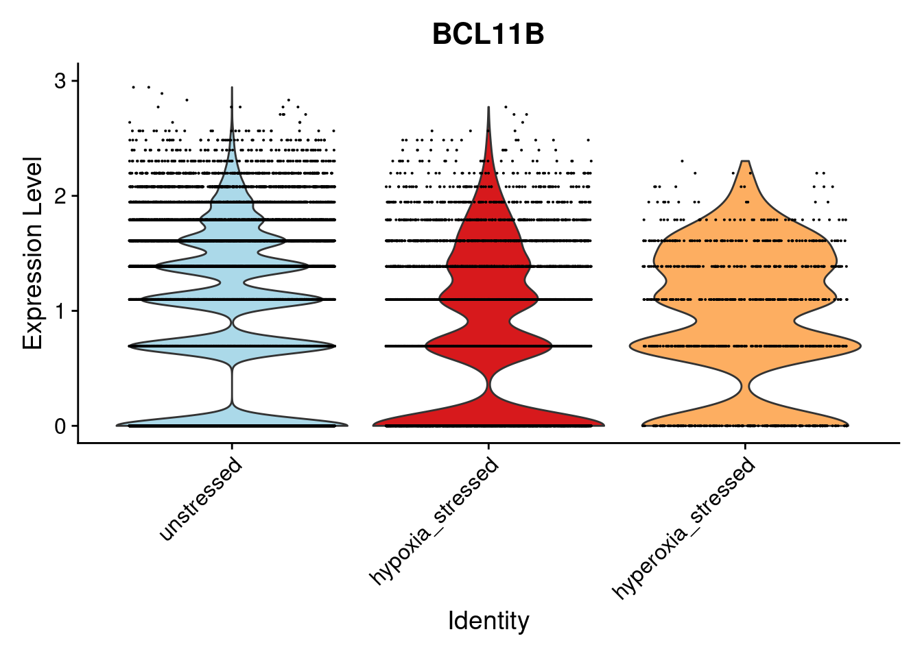

VlnPlot(immature_subset, features = "MAP2", group.by = "gruffi_label_mash", y.max=3, cols=colors) + NoLegend()

Warning: Removed 61 rows containing non-finite values (`stat_ydensity()`).

Warning: Removed 61 rows containing missing values (`geom_point()`).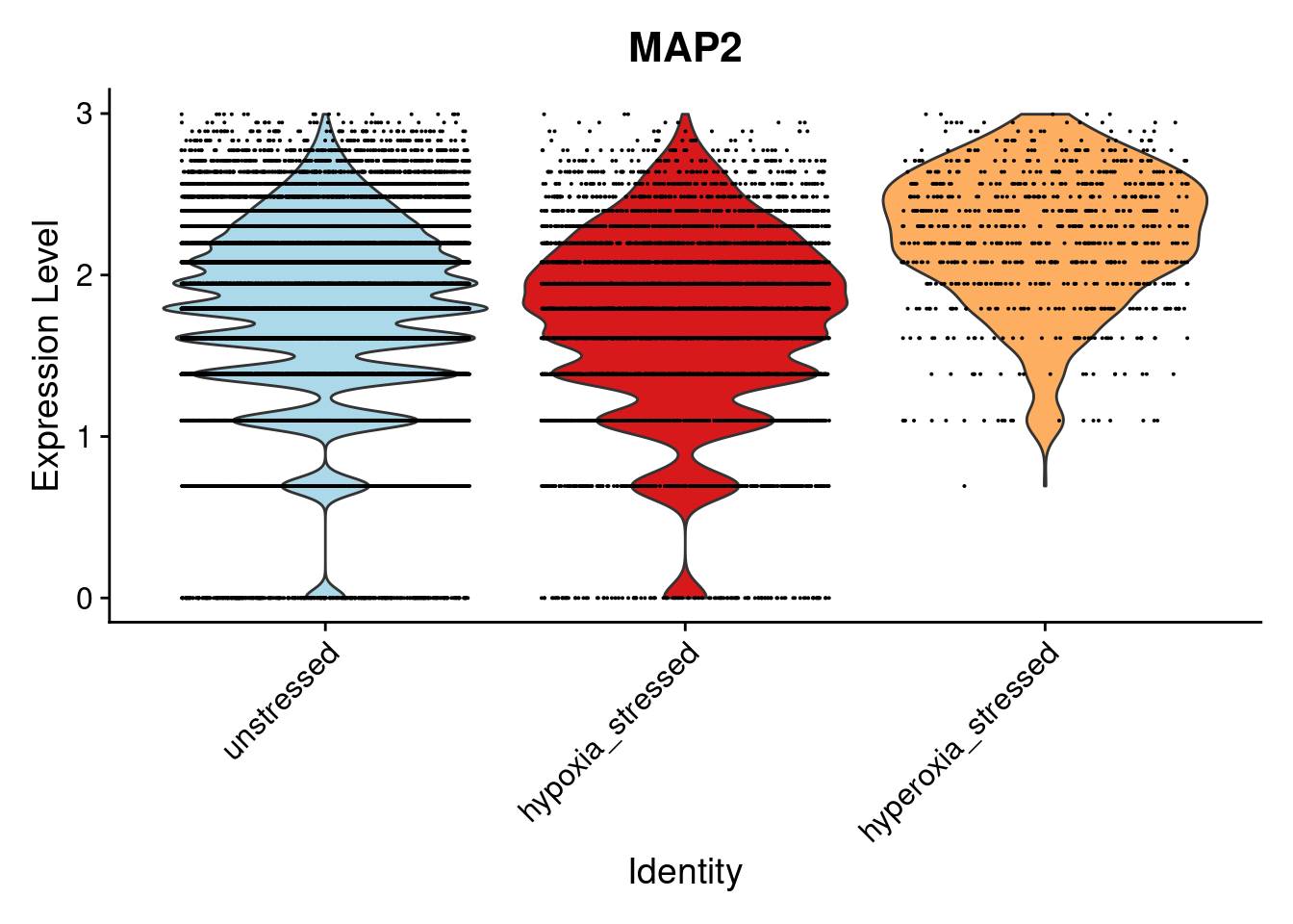

VlnPlot(immature_subset, features = "SLA", group.by = "gruffi_label_mash", y.max=3, cols=colors) + NoLegend()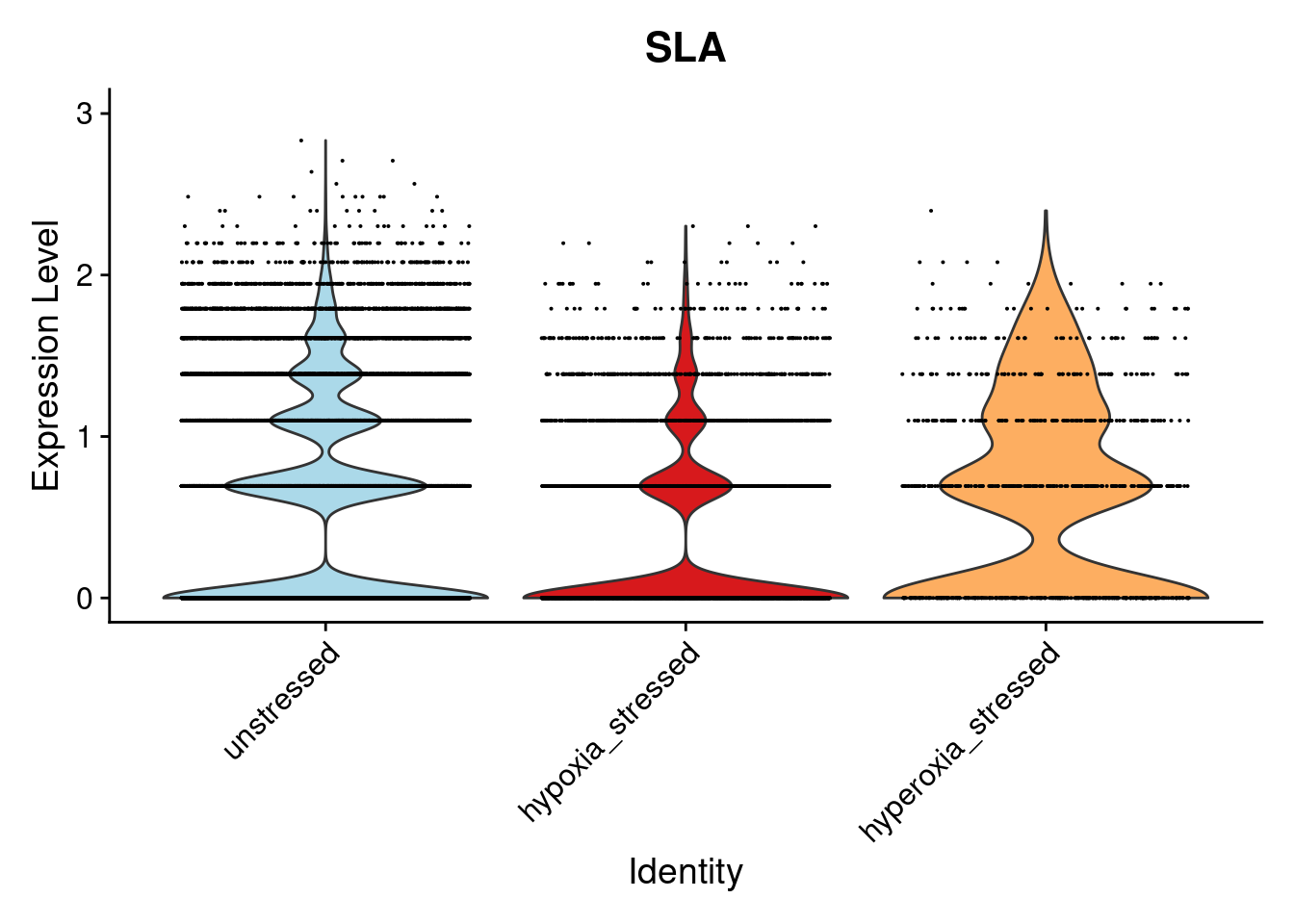

DE with Gruffi-flagged cells censored

harmony.batchandindividual.sct.censored <- subset(harmony.batchandindividual.sct, subset = gruffi_label_mash=="unstressed")

Now filter to “high quality” cells and pseudobulk. This time, however, don’t use the cell type mapping threshold, as this penalizes “ambiguous” cell types, which makes sense for QTL mapping but not so much for the DE here. Note that this does not have a treatment bias, thankfully.

subset_seurat_censored <- subset(harmony.batchandindividual.sct.censored, subset = vireo.prob.singlet > 0.95 & nCount_RNA<20000 & nCount_RNA>2500 & treatment != "control21")

subset_seurat <- subset(harmony.batchandindividual.sct, subset = vireo.prob.singlet > 0.95 & nCount_RNA<20000 & nCount_RNA>2500 & treatment != "control21" )

We originally used with:

table(subset_seurat$treatment)

control10  stim1pct stim21pct 
    52671     57788     60382 

And now have

table(subset_seurat_censored$treatment)

control10  stim1pct stim21pct 
    47817     39629     54676 

control10 stim1pct stim21pct 47817 39629 56173

This censors about 9% of the control cells, 31% of the hypoxia cells, and 7% of the hyperoxia cells, about 16% of the total dataset.

pseudo_fine_quality_censored <- generate.pseudobulk(subset_seurat_censored, labels = c("combined.annotation.fine.harmony", "treatment", "vireo.individual", "batch"))
saveRDS(pseudo_fine_quality_censored, file = "/project2/gilad/umans/oxygen_eqtl/output/pseudo_fine_quality_filtered_de_censored_20240802.RDS")

pseudo_fine_quality_censored <- readRDS(file = "/project2/gilad/umans/oxygen_eqtl/output/pseudo_fine_quality_filtered_de_censored_20240802.RDS")
pseudo_fine_quality_de_censored <- filter.pseudobulk(pseudo_fine_quality_censored, threshold = 20)

pseudo_fine_quality_de_censored$counts <- pseudo_fine_quality_de_censored$counts[,-c(which(pseudo_fine_quality_de_censored$meta$combined.annotation.fine.harmony=="Oligo"))]
pseudo_fine_quality_de_censored$meta <- pseudo_fine_quality_de_censored$meta %>% filter(combined.annotation.fine.harmony != "Oligo")

# pseudo_fine_quality_de_censored$counts <- pseudo_fine_quality_de_censored$counts[,-c(which(pseudo_fine_quality_de_censored$meta$combined.annotation.fine.harmony=="MidbrainDA"))]
# pseudo_fine_quality_de_censored$meta <- pseudo_fine_quality_de_censored$meta %>% filter(combined.annotation.fine.harmony != "MidbrainDA")

pseudo_fine_quality_de_censored$counts <- pseudo_fine_quality_de_censored$counts[,-c(which(pseudo_fine_quality_de_censored$meta$combined.annotation.fine.harmony=="VLMC"))]
pseudo_fine_quality_de_censored$meta <- pseudo_fine_quality_de_censored$meta %>% filter(combined.annotation.fine.harmony != "VLMC")

de_results_combinedfine_filtered_censored <- de_genes_pseudoinput(pseudo_input = pseudo_fine_quality_de_censored, classification = "combined.annotation.fine.harmony", model_formula = model_formula, maineffect = "treatment", min.count = 5, min.prop=0.7, min.total.count = 10)

saveRDS(de_results_combinedfine_filtered_censored, file = "/project2/gilad/umans/oxygen_eqtl/output/de_results_combinedfine_filtered_reharmonize_censored_20240802.RDS")

Of course, downsampling the data will result in fewer DE genes, so I compare this to a random downsampling of the same proportions from the different conditions:

censoring_stats_hypoxia <- subset_seurat@meta.data %>% 
  filter(gruffi_label_mash != "hyperoxia_stressed") %>% 
  group_by(combined.annotation.fine.harmony) %>% 
  summarize(fraction=sum(gruffi_label_mash=="hypoxia_stressed")/n()) 

censoring_stats_hyperoxia <- subset_seurat@meta.data %>% 
  filter(gruffi_label_mash != "hypoxia_stressed") %>% 
  group_by(combined.annotation.fine.harmony) %>% 
  summarize(fraction=sum(gruffi_label_mash=="hyperoxia_stressed")/n()) 

subset_seurat$selection <- NA

for (celltype in censoring_stats_hypoxia$combined.annotation.fine.harmony){
  indices_hypoxia <- sample(x = which(subset_seurat$combined.annotation.fine.harmony==celltype), size = round(deframe(censoring_stats_hypoxia)[celltype]*length(which(subset_seurat$combined.annotation.fine.harmony==celltype))), replace = FALSE)
  
  indices_hyperoxia <- sample(x = which(subset_seurat$combined.annotation.fine.harmony==celltype), size = round(deframe(censoring_stats_hyperoxia)[celltype]*length(which(subset_seurat$combined.annotation.fine.harmony==celltype))), replace = FALSE)
  
  subset_seurat$selection[unique(c(indices_hypoxia, indices_hyperoxia))] <- "random_censored"
  
  rm(indices_hypoxia, indices_hyperoxia)
}

subset_seurat_censored_random <- subset(subset_seurat, subset = selection == "random_censored", invert=TRUE)

pseudo_fine_quality_censored_random <- generate.pseudobulk(subset_seurat_censored_random, labels = c("combined.annotation.fine.harmony", "treatment", "vireo.individual", "batch"))
saveRDS(pseudo_fine_quality_censored_random, file = "output/pseudo_fine_quality_filtered_de_randomly_censored_20240802.RDS")

pseudo_fine_quality_censored_random <- readRDS(file = "/project2/gilad/umans/oxygen_eqtl/output/pseudo_fine_quality_filtered_de_randomly_censored_20240802.RDS")
pseudo_fine_quality_de_censored_random <- filter.pseudobulk(pseudo_fine_quality_censored_random, threshold = 20)

pseudo_fine_quality_de_censored_random$counts <- pseudo_fine_quality_de_censored_random$counts[,-c(which(pseudo_fine_quality_de_censored_random$meta$combined.annotation.fine.harmony=="Oligo"))]
pseudo_fine_quality_de_censored_random$meta <- pseudo_fine_quality_de_censored_random$meta %>% filter(combined.annotation.fine.harmony != "Oligo")

pseudo_fine_quality_de_censored_random$counts <- pseudo_fine_quality_de_censored_random$counts[,-c(which(pseudo_fine_quality_de_censored_random$meta$combined.annotation.fine.harmony=="VLMC"))]
pseudo_fine_quality_de_censored_random$meta <- pseudo_fine_quality_de_censored_random$meta %>% filter(combined.annotation.fine.harmony != "VLMC")

de_results_combinedfine_filtered_censored_random <- de_genes_pseudoinput(pseudo_input = pseudo_fine_quality_de_censored_random, classification = "combined.annotation.fine.harmony", model_formula = model_formula, maineffect = "treatment", min.count = 5, min.prop=0.7, min.total.count = 10)

saveRDS(de_results_combinedfine_filtered_censored_random, file = "/project2/gilad/umans/oxygen_eqtl/output/de_results_combinedfine_filtered_reharmonize_random_censored_20240802.RDS")

de_results_combinedfine_filtered_censored_random <- readRDS(file = "/project2/gilad/umans/oxygen_eqtl/output/de_results_combinedfine_filtered_reharmonize_random_censored_20240802.RDS")

de_results_combinedfine_filtered_censored <- readRDS(file = "/project2/gilad/umans/oxygen_eqtl/output/de_results_combinedfine_filtered_reharmonize_censored_20240802.RDS")

Summarize the results, looking at the change between the randomly censored and stress-censored:

# here, the "uncensored" are the randomly censored, in order to match number of individuals

de.summary.fine.censored.change.random <-  matrix(0, nrow = length(names(de_results_combinedfine_filtered_censored_random)), ncol =10)
colnames(de.summary.fine.censored.change.random) <-c("hypoxia_random_censored", "hyperoxia_random_censored", "hypoxia_censored", "hyperoxia_censored", "nindiv_hypoxia", "nindiv_hyperoxia", "hypoxia_mineffect_random_censored", "hyperoxia_mineffect_random_censored", "hypoxia_mineffect_censored", "hyperoxia_mineffect_censored")
rownames(de.summary.fine.censored.change.random) <- names(de_results_combinedfine_filtered_censored_random)


for (cell in names(de_results_combinedfine_filtered_censored_random)){
    de.summary.fine.censored.change.random[cell, 1] <- sum(topTable(de_results_combinedfine_filtered_censored_random[[cell]], coef="treatmentstim1pct", number = Inf)$adj.P.Val < 0.05)
  de.summary.fine.censored.change.random[cell, 2] <- sum(topTable(de_results_combinedfine_filtered_censored_random[[cell]], coef="treatmentstim21pct", number = Inf)$adj.P.Val < 0.05)
    de.summary.fine.censored.change.random[cell, 3] <- sum(topTable(de_results_combinedfine_filtered_censored[[cell]], coef="treatmentstim1pct", number = Inf)$adj.P.Val < 0.05)
  de.summary.fine.censored.change.random[cell, 4] <- sum(topTable(de_results_combinedfine_filtered_censored[[cell]], coef="treatmentstim21pct", number = Inf)$adj.P.Val < 0.05)
  

    de.summary.fine.censored.change.random[cell, 5] <- pseudo_fine_quality_de_censored$meta %>% filter(combined.annotation.fine.harmony==cell) %>% dplyr::filter(treatment %in% c("control10", "stim1pct")) %>% pull(vireo.individual) %>% unique() %>% length()
    de.summary.fine.censored.change.random[cell, 6] <- pseudo_fine_quality_de_censored$meta %>% filter(combined.annotation.fine.harmony==cell) %>% dplyr::filter(treatment %in% c("control10", "stim21pct")) %>% pull(vireo.individual) %>% unique() %>% length()
    de.summary.fine.censored.change.random[cell, 7] <- topTable(de_results_combinedfine_filtered_censored_random[[cell]], coef="treatmentstim1pct", number = Inf) %>% filter(adj.P.Val < 0.05) %>% filter(abs(logFC)>0.58) %>% nrow() 
  de.summary.fine.censored.change.random[cell, 8] <- topTable(de_results_combinedfine_filtered_censored_random[[cell]], coef="treatmentstim21pct", number = Inf) %>% filter(adj.P.Val < 0.05) %>% filter(abs(logFC)>0.58) %>% nrow()

    de.summary.fine.censored.change.random[cell, 9] <- topTable(de_results_combinedfine_filtered_censored[[cell]], coef="treatmentstim1pct", number = Inf) %>% filter(adj.P.Val < 0.05) %>% filter(abs(logFC)>0.58) %>% nrow() 
  de.summary.fine.censored.change.random[cell, 10] <- topTable(de_results_combinedfine_filtered_censored[[cell]], coef="treatmentstim21pct", number = Inf) %>% filter(adj.P.Val < 0.05) %>% filter(abs(logFC)>0.58) %>% nrow()

}

de.summary.fine.censored.change.random <- de.summary.fine.censored.change.random %>% as.data.frame() %>% arrange(nindiv_hypoxia) %>% rownames_to_column("celltype")

de.summary.fine.censored.change.random %>% 
  left_join(y = censoring_stats_hypoxia, by=join_by(celltype==combined.annotation.fine.harmony)) %>% 
  ggplot(mapping = aes(x=fraction, y=1-(hypoxia_mineffect_censored/hypoxia_mineffect_random_censored), label=celltype)) +
  geom_point() + geom_text_repel() + 
  theme_light() + 
  xlab("Censored fraction") + 
  ylab("1-(stress-censored DE genes/randomly censored DE genes)") + geom_abline(slope = 1, intercept = 0, linetype=2) +
  ggtitle("hypoxia >1.5fold")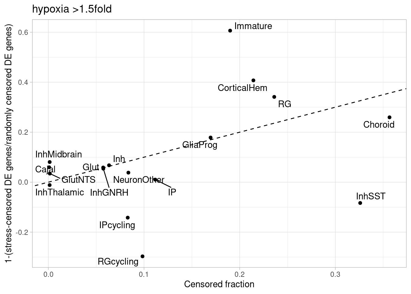

Cell positions within organoids

Here, I import measurement information from QuPath, classify cells as positive for stained markers (thresholds were identified iteratively by comparisons using QuPath), and combine results from different staining sets.

For samples stained for HOPX/KI67/S100b:

annotations_hopx <- read_delim(file =  "HOPX_MKI67_S100B/QuPath_output/Stardist_measurements_HOPX_MKI67_S100B_annotations.csv") %>% 
  filter(Name != "Other") %>% 
  dplyr::select(Image, `Object ID`, Name, `Area µm^2`, `Perimeter µm`)
hopx1 <- read_delim(file =  "HOPX_MKI67_S100B/QuPath_output/Stardist_measurements_HOPX_MKI67_S100B_detections1.csv")
hopx2 <- read_delim(file =  "HOPX_MKI67_S100B/QuPath_output/Stardist_measurements_HOPX_MKI67_S100B_detections2.csv")
hopx3 <- read_delim(file =  "HOPX_MKI67_S100B/QuPath_output/Stardist_measurements_HOPX_MKI67_S100B_detections3.csv")

detections_hopx <- bind_rows(hopx1, hopx2, hopx3) %>% left_join(annotations_hopx, by=c("Parent" = "Name"))
rm(hopx1, hopx2, hopx3)

detections_hopx_plotting <- detections_hopx %>% 
  replace_na(list(`MCherry: Nucleus: Mean`=0, `TRITC: Nucleus: Mean`=0)) %>% ##DEAL WITH NAs for >
  group_by(Parent) %>% 
  mutate(HOPX= `FITC: Nucleus: Mean` >  mean(`FITC: Nucleus: Mean`) + 2*sd(`FITC: Nucleus: Mean`)) %>% 
  mutate(MKI67 = (`MCherry: Nucleus: Mean` > mean(`MCherry: Nucleus: Mean`) + 1.5*sd(`MCherry: Nucleus: Mean`)) | (`TRITC: Nucleus: Mean` > mean(`TRITC: Nucleus: Mean`) + 1.5*sd(`TRITC: Nucleus: Mean`))) %>% 
  mutate(S100B = `Cy5: Nucleus: Mean` > mean(`Cy5: Nucleus: Mean`) + 2*sd(`Cy5: Nucleus: Mean`)) %>% 
  ungroup() %>% 
  mutate(scaled_distance= `Distance to annotation with Other µm`/sqrt(`Area µm^2`)) 

df <- detections_hopx_plotting %>% select(HOPX, MKI67, S100B)
detections_hopx_plotting$cell_type <-apply(df, 1, function(x) paste(names(df)[x], collapse = ","))

rm(df)

For samples stained for EOMES/CTIP2/SATB2:

annotations_eomes <- read_delim(file =  "EOMES_CTIP2_SATB2/QuPath_output/Stardist_measurements_EOMES_CTIP2_SATB2_annotations.csv") %>% 
  filter(Name != "Other") %>% 
  dplyr::select(Image, `Object ID`, Name, `Area µm^2`, `Perimeter µm`)

eomes1 <- read_delim(file =  "EOMES_CTIP2_SATB2/QuPath_output/Stardist_measurements_EOMES_CTIP2_SATB2_detections1.csv") 
eomes2 <- read_delim(file =  "EOMES_CTIP2_SATB2/QuPath_output/Stardist_measurements_EOMES_CTIP2_SATB2_detections2.csv") 
eomes3 <- read_delim(file =  "EOMES_CTIP2_SATB2/QuPath_output/Stardist_measurements_EOMES_CTIP2_SATB2_detections3.csv") 

detections_eomes <- bind_rows(eomes1, eomes2, eomes3) %>% left_join(annotations_eomes, by=c("Parent" = "Name"))

rm(eomes1, eomes2, eomes3)

detections_eomes_plotting <- detections_eomes %>% 
  group_by(Parent) %>% 
  mutate(EOMES= `FITC: Nucleus: Mean` >  mean(`FITC: Nucleus: Mean`) + 1.5*sd(`FITC: Nucleus: Mean`)) %>% 
  mutate(SATB2 = `TRITC: Nucleus: Mean` > mean(`TRITC: Nucleus: Mean`) + 1.5*sd(`TRITC: Nucleus: Mean`) ) %>% 
  mutate(CTIP2 = `Cy5: Nucleus: Mean` > max(mean(`Cy5: Nucleus: Mean`) + 1*sd(`Cy5: Nucleus: Mean`), 1300)) %>% 
  ungroup() %>% 
  mutate(scaled_distance= `Distance to annotation with Other µm`/sqrt(`Area µm^2`)) 

df <- detections_eomes_plotting %>% select(EOMES, SATB2, CTIP2)
detections_eomes_plotting$cell_type <-apply(df, 1, function(x) paste(names(df)[x], collapse = ","))

rm(df)

For samples stained for RELN/GABA/CTIP2:

annotations_reln <- read_delim(file =  "RELN_GABA_CTIP2/QuPath_output/Stardist_measurements_RELN_GABA_CTIP2_annotations.csv") %>% 
  filter(Name != "Other") %>% 
  dplyr::select(Image, `Object ID`, Name, `Area µm^2`, `Perimeter µm`)

reln1 <- read_delim(file =  "RELN_GABA_CTIP2/QuPath_output/Stardist_measurements_RELN_GABA_CTIP2_detections1.csv") 
reln2 <- read_delim(file =  "RELN_GABA_CTIP2/QuPath_output/Stardist_measurements_RELN_GABA_CTIP2_detections2.csv") 

detections_reln <- bind_rows(reln1, reln2) %>% left_join(annotations_reln, by=c("Parent" = "Name"))

rm(reln1, reln2)

detections_reln_plotting <- detections_reln %>% 
  group_by(Parent) %>% 
  mutate(RELN= `FITC: Nucleus: Mean` >  max(mean(`FITC: Nucleus: Mean`) + 2*sd(`FITC: Nucleus: Mean`), 1100)) %>% 
  mutate(GABA = `MCherry: Nucleus: Mean` > max(mean(`MCherry: Nucleus: Mean`) + 2*sd(`MCherry: Nucleus: Mean`), 1000)) %>% 
  mutate(CTIP2 = `Cy5: Nucleus: Mean` > mean(`Cy5: Nucleus: Mean`) + 1.5*sd(`Cy5: Nucleus: Mean`)) %>% 
  ungroup() %>% 
  mutate(scaled_distance= `Distance to annotation with Other µm`/sqrt(`Area µm^2`)) 

df <- detections_reln_plotting %>% select(RELN, GABA, CTIP2)
detections_reln_plotting$cell_type <-apply(df, 1, function(x) paste(names(df)[x], collapse = ","))

detections_reln_plotting_singlesection <- detections_reln_plotting %>% group_by(cell_line, BP) %>% 
  filter(`Area µm^2`==max(`Area µm^2`)) %>% ungroup()
rm(df)

For samples stained for SOX2/NES/S100B:

annotations_sox <- read_delim(file =  "SOX2_NES_S100B/QuPath_output/Stardist_measurements_SOX2_NES_S100B_annotations.csv") %>% 
  filter(Name != "Other") %>% 
  dplyr::select(Image, `Object ID`, Name, `Area µm^2`, `Perimeter µm`)

sox1 <- read_delim(file =  "SOX2_NES_S100B/QuPath_output/Stardist_measurements_SOX2_NES_S100B_detections1.csv") 
sox2 <- read_delim(file =  "SOX2_NES_S100B/QuPath_output/Stardist_measurements_SOX2_NES_S100B_detections2.csv") 
sox3 <- read_delim(file =  "SOX2_NES_S100B/QuPath_output/Stardist_measurements_SOX2_NES_S100B_detections3.csv") 
sox4 <- read_delim(file =  "SOX2_NES_S100B/QuPath_output/Stardist_measurements_SOX2_NES_S100B_detections4.csv") 

detections_sox <- bind_rows(sox1, sox2, sox3, sox4) %>% left_join(annotations_sox, by=c("Parent" = "Name"))

rm(sox1, sox2, sox3, sox4)

detections_sox_plotting <- detections_sox %>% 
  group_by(Parent) %>% 
  mutate(SOX2= `FITC: Nucleus: Mean` >  max(mean(`FITC: Nucleus: Mean`) + 1*sd(`FITC: Nucleus: Mean`), 800)) %>% 
  mutate(NES= `TRITC: Nucleus: Mean` > mean(`TRITC: Nucleus: Mean`) + 1*sd(`TRITC: Nucleus: Mean`)) %>% 
  mutate(S100B = `Cy5: Nucleus: Mean` > mean(`Cy5: Nucleus: Mean`) + 1*sd(`Cy5: Nucleus: Mean`)) %>% 
  ungroup() %>% 
  mutate(scaled_distance= `Distance to annotation with Other µm`/sqrt(`Area µm^2`)) 

df <- detections_sox_plotting %>% select(SOX2, NES, S100B)
detections_sox_plotting$cell_type <-apply(df, 1, function(x) paste(names(df)[x], collapse = ","))


detections_sox_plotting_singlesection <- detections_sox_plotting %>% group_by(cell_line, BP) %>% 
  filter(`Area µm^2`==max(`Area µm^2`)) %>% ungroup()

rm(df)

For samples stained for GFAP:

annotations_gfap <- read_delim(file =  "MGP_GFAP/QuPath_output/Stardist_measurements_MGP_GFAP_annotations.csv") %>% 
  filter(Name != "Other") %>% 
  dplyr::select(Image, `Object ID`, Name, `Area µm^2`, `Perimeter µm`)

gfap1 <- read_delim(file =  "MGP_GFAP/QuPath_output/Stardist_measurements_MGP_GFAP_detections1.csv") 
gfap2 <- read_delim(file =  "MGP_GFAP/QuPath_output/Stardist_measurements_MGP_GFAP_detections2.csv") 

detections_gfap <- bind_rows(gfap1, gfap2) %>% left_join(annotations_gfap, by=c("Parent" = "Name"))

rm(gfap1, gfap2)

detections_gfap_plotting <- detections_gfap %>% 
  group_by(Parent) %>% 
  mutate(GFAP = `Cy5: Nucleus: Mean` > mean(`Cy5: Nucleus: Mean`) + 1.5*sd(`Cy5: Nucleus: Mean`)) %>% 
  ungroup() %>% 
  mutate(scaled_distance= `Distance to annotation with Other µm`/sqrt(`Area µm^2`)) 

df <- detections_gfap_plotting %>% select(GFAP)
detections_gfap_plotting$cell_type <-apply(df, 1, function(x) paste(names(df)[x], collapse = ","))

detections_gfap_plotting_singlesection <- detections_gfap_plotting %>% group_by(cell_line, BP) %>% 
  filter(`Area µm^2`==max(`Area µm^2`)) %>% ungroup()

rm(df)

Combine all of the data:

combined_plotting_singlesection <- bind_rows(detections_reln_plotting_singlesection %>% select(cell_line, Parent, BP, scaled_distance, `Distance to annotation with Other µm`, cell_type),
                                             detections_sox_plotting_singlesection %>% select(cell_line, Parent, BP, scaled_distance, `Distance to annotation with Other µm`, cell_type),
                                             detections_reln_plotting_singlesection %>% select(cell_line, Parent, BP, scaled_distance, `Distance to annotation with Other µm`, cell_type),
                                             detections_gfap_plotting_singlesection %>% select(cell_line, Parent, BP, scaled_distance, `Distance to annotation with Other µm`, cell_type),
                                             detections_eomes_plotting_singlesection %>% select(cell_line, Parent, BP, scaled_distance, `Distance to annotation with Other µm`, cell_type),
                                             detections_hopx_plotting_singlesection %>% select(cell_line, Parent, BP, scaled_distance, `Distance to annotation with Other µm`, cell_type)) %>% 
  mutate_at("cell_type", ~na_if(., "")) %>% 
  mutate(cell_type=replace_na(cell_type, "unlabeled"))

Cell types were classified based on the stained markers in combination within a given staining set, as not all cells can be distinguished in each context (e.g., CTIP2+ neurons can only be distinguished from SATB2+/CTIP2+ neurons when both antibodies are present).

combined_plotting_singlesection$cell_type_pooled_revised <- "unlabeled"

combined_plotting_singlesection <- combined_plotting_singlesection %>% mutate(cell_type_pooled_revised =case_when(
  str_detect(Parent, "CTIP2_SATB2") & cell_type=="CTIP2" ~ "Excitatory-early",
  str_detect(Parent, "CTIP2_SATB2") & cell_type=="SATB2" ~ "Excitatory-late",
  str_detect(Parent, "CTIP2_SATB2") & cell_type=="SATB2,CTIP2" ~ "Excitatory-late",
  str_detect(Parent, "CTIP2_SATB2") & cell_type=="EOMES" ~ "IP",
  str_detect(Parent, "HOPX") & cell_type=="MKI67" ~ "DividingProgenitors",
  str_detect(Parent, "HOPX") & cell_type=="HOPX" ~ "RadialGlia",
  str_detect(Parent, "HOPX") & cell_type=="HOPX,MKI67" ~ "RadialGlia",
  str_detect(Parent, "HOPX") & cell_type=="S100B" ~ "Glia",
  str_detect(Parent, "RELN") & cell_type=="RELN" ~ "Cajal",
  str_detect(Parent, "RELN") & cell_type=="RELN,GABA" ~ "Inhibitory",
  str_detect(Parent, "RELN") & cell_type=="GABA" ~ "Inhibitory",
  str_detect(Parent, "RELN") & cell_type=="GABA,CTIP2" ~ "Inhibitory",  #we ignore the large number of CTIP2+/GABA- cells here because we can't distinguish them from the substantial number of CTIP2+/SATB2+ (ie, "mature") excitatory neurons
  str_detect(Parent, "SOX2_NES_S100b") & cell_type=="SOX2,NES,S100B" ~ "Glia",
  str_detect(Parent, "SOX2_NES_S100b") & cell_type=="S100B" ~ "Glia", #while this marker is not perfect in many in vivo contexts, the correspondence is clear in our RNAseq data
  # str_detect(Parent, "SOX2_NES_S100b") & cell_type=="SOX2,S100B" ~ "RadialGlia",
  str_detect(Parent, "SOX2_NES_S100b") & cell_type=="SOX2,NES" ~ "OtherProgenitor", #NES should mark Glia, Floorplate, RG, Cycling Progenitors; S100B should be (RNA) specific for Glia; SOX2 hits choroid/cycling progenitors/floorplate/glia/IP/RG
  str_detect(Parent, "GFAP") & cell_type=="GFAP" ~ "Glia", #again, while this marker is not perfect in many in vivo contexts, the correspondence is clear in our RNAseq data
  .default="unlabeled"))

For plotting purposes, load the processed data object:

combined_plotting_singlesection <- readRDS(file = "/project2/gilad/umans/oxygen_eqtl/output/combined_plotting_singlesection_upload.RDS")

Next, plot the distributions of cell types here. Note that, as this is intended as a comparison for responsive cell types as annotated in our single-cell RNAseq data, we exclude cells (e.g., “other progenitors”) that do not have a specific correspondence in our transcriptomic data:

positions <- c( #"DividingProgenitors",
               "IP",
               "Excitatory-early",
               "RadialGlia",
               "Excitatory-late",
               "Inhibitory",
               "Glia",
               "Cajal",
               "unlabeled"
              )

color_set <- c("unlabeled"= "black",
               "DividingProgenitors"="#882255",
               "RadialGlia"="#8DD3C7", 
               "Cajal"="#80B1D3",
               "IP"="#BEBADA", 
               "Excitatory-early"="#FB8072",
               "Excitatory-late"="#fc9016",
               "Excitatory"="#88CCEE",
               "Inhibitory"="#AFAFAF", 
               "Glia"="#FFFFB3")


ggplot(combined_plotting_singlesection, aes(x=cell_type_pooled_revised, y=`Distance to annotation with Other µm`, color=cell_type_pooled_revised)) + geom_boxplot(linewidth=0.4, outlier.size = 0.5) + scale_x_discrete(limits = positions) + 
  ggtitle("Cell distances, aggregated over individuals") +
  scale_colour_manual(values = color_set) +
  stat_summary(fun.y = median, 
               geom = "point",
               aes(group = interaction(Parent, cell_type_pooled_revised)),
               size = 0.5, show.legend = F, color="black") + 
  theme_light() + theme(legend.position="none") + coord_flip()

Warning: The `fun.y` argument of `stat_summary()` is deprecated as of ggplot2 3.3.0.
ℹ Please use the `fun` argument instead.
This warning is displayed once every 8 hours.
Call `lifecycle::last_lifecycle_warnings()` to see where this warning was
generated.

Warning: Removed 18710 rows containing missing values (`stat_boxplot()`).

Warning: Removed 18710 rows containing non-finite values (`stat_summary()`).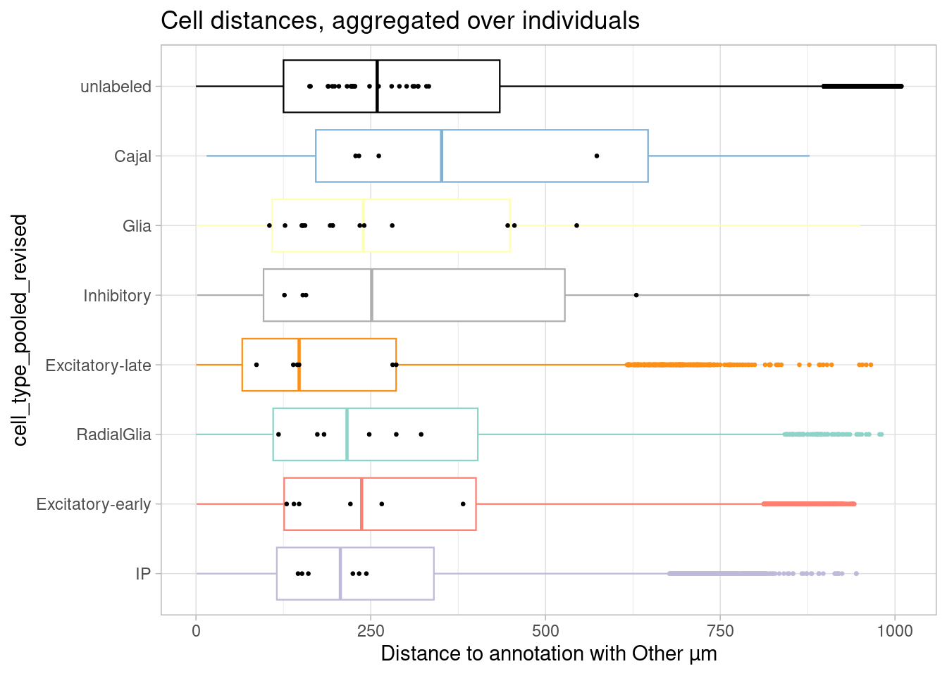

There are, of course, differences between cell types when all aggregated together. To compare the differences between individuals to the differences between cell types, we can use ANOVA, using the mean values for cells within each sample (ie, individual).

aov_test <- aov(data ~ cell_type_pooled_revised, data = combined_plotting_singlesection %>% 
                  group_by(Parent, cell_type_pooled_revised) %>% 
                  summarise(data=mean(`Distance to annotation with Other µm`)) %>% 
                  ungroup())

`summarise()` has grouped output by 'Parent'. You can override using the
`.groups` argument.
`summarise()` has grouped output by 'Parent'. You can override using the
`.groups` argument.

summary(aov_test)

                         Df Sum Sq Mean Sq F value Pr(>F)
cell_type_pooled_revised  9  64006    7112   0.783  0.632
Residuals                76 690016    9079               

And we can do this with each post-hoc comparison for further detail:

library(afex)

Loading required package: lme4

Loading required package: Matrix

Attaching package: 'Matrix'

The following objects are masked from 'package:tidyr':

    expand, pack, unpack

************
Welcome to afex. For support visit: http://afex.singmann.science/

- Functions for ANOVAs: aov_car(), aov_ez(), and aov_4()
- Methods for calculating p-values with mixed(): 'S', 'KR', 'LRT', and 'PB'
- 'afex_aov' and 'mixed' objects can be passed to emmeans() for follow-up tests
- Get and set global package options with: afex_options()
- Set sum-to-zero contrasts globally: set_sum_contrasts()
- For example analyses see: browseVignettes("afex")
************

Attaching package: 'afex'

The following object is masked from 'package:lme4':

    lmer

library(emmeans)
summarized_data <- combined_plotting_singlesection %>% group_by(Parent, cell_type_pooled_revised) %>% summarise(data=mean(`Distance to annotation with Other µm`)) %>% ungroup() %>% mutate(id=row_number())

`summarise()` has grouped output by 'Parent'. You can override using the
`.groups` argument.

aovcar_test <- aov_car(formula = data ~ cell_type_pooled_revised + Error(id), data = summarized_data)

Converting to factor: cell_type_pooled_revised

Contrasts set to contr.sum for the following variables: cell_type_pooled_revised

pairs(emmeans(aovcar_test, specs = "cell_type_pooled_revised"))

 contrast                                 estimate   SE df t.ratio p.value
 Cajal - DividingProgenitors                79.881 61.5 76   1.299  0.9510
 Cajal - (Excitatory-early)                 58.683 61.5 76   0.954  0.9939
 Cajal - (Excitatory-late)                  84.754 61.5 76   1.378  0.9302
 Cajal - Glia                               54.534 53.3 76   1.024  0.9899
 Cajal - IP                                 95.881 61.5 76   1.559  0.8631
 Cajal - Inhibitory                         22.879 67.4 76   0.340  1.0000
 Cajal - OtherProgenitor                   109.040 61.5 76   1.773  0.7497
 Cajal - RadialGlia                         58.060 61.5 76   0.944  0.9944
 Cajal - unlabeled                          34.351 51.2 76   0.671  0.9996
 DividingProgenitors - (Excitatory-early)  -21.198 55.0 76  -0.385  1.0000
 DividingProgenitors - (Excitatory-late)     4.873 55.0 76   0.089  1.0000
 DividingProgenitors - Glia                -25.346 45.6 76  -0.556  0.9999
 DividingProgenitors - IP                   16.001 55.0 76   0.291  1.0000
 DividingProgenitors - Inhibitory          -57.002 61.5 76  -0.927  0.9951
 DividingProgenitors - OtherProgenitor      29.159 55.0 76   0.530  0.9999
 DividingProgenitors - RadialGlia          -21.821 55.0 76  -0.397  1.0000
 DividingProgenitors - unlabeled           -45.530 43.2 76  -1.055  0.9875
 (Excitatory-early) - (Excitatory-late)     26.071 55.0 76   0.474  1.0000
 (Excitatory-early) - Glia                  -4.148 45.6 76  -0.091  1.0000
 (Excitatory-early) - IP                    37.199 55.0 76   0.676  0.9996
 (Excitatory-early) - Inhibitory           -35.804 61.5 76  -0.582  0.9999
 (Excitatory-early) - OtherProgenitor       50.357 55.0 76   0.915  0.9955
 (Excitatory-early) - RadialGlia            -0.623 55.0 76  -0.011  1.0000
 (Excitatory-early) - unlabeled            -24.332 43.2 76  -0.564  0.9999
 (Excitatory-late) - Glia                  -30.219 45.6 76  -0.663  0.9996
 (Excitatory-late) - IP                     11.128 55.0 76   0.202  1.0000
 (Excitatory-late) - Inhibitory            -61.875 61.5 76  -1.006  0.9911
 (Excitatory-late) - OtherProgenitor        24.286 55.0 76   0.441  1.0000
 (Excitatory-late) - RadialGlia            -26.694 55.0 76  -0.485  1.0000
 (Excitatory-late) - unlabeled             -50.403 43.2 76  -1.168  0.9750
 Glia - IP                                  41.347 45.6 76   0.906  0.9958
 Glia - Inhibitory                         -31.656 53.3 76  -0.594  0.9999
 Glia - OtherProgenitor                     54.505 45.6 76   1.195  0.9710
 Glia - RadialGlia                           3.525 45.6 76   0.077  1.0000
 Glia - unlabeled                          -20.184 30.3 76  -0.667  0.9996
 IP - Inhibitory                           -73.003 61.5 76  -1.187  0.9722
 IP - OtherProgenitor                       13.158 55.0 76   0.239  1.0000
 IP - RadialGlia                           -37.822 55.0 76  -0.688  0.9995
 IP - unlabeled                            -61.531 43.2 76  -1.426  0.9152
 Inhibitory - OtherProgenitor               86.161 61.5 76   1.401  0.9233
 Inhibitory - RadialGlia                    35.181 61.5 76   0.572  0.9999
 Inhibitory - unlabeled                     11.472 51.2 76   0.224  1.0000
 OtherProgenitor - RadialGlia              -50.980 55.0 76  -0.927  0.9951
 OtherProgenitor - unlabeled               -74.689 43.2 76  -1.731  0.7746
 RadialGlia - unlabeled                    -23.709 43.2 76  -0.549  0.9999

P value adjustment: tukey method for comparing a family of 10 estimates 

(Note that summarizing by median produces a qualitatively equivalent result).

Keeping in mind that the main result of the ANOVA is that inter-individual variation is large enough to prevent making stable conclusions about systematic differences in cell type positions across many samples, we can compare the average cell type distances and responses to hypoxia (plotted above) and confirm a lack of correlation:

temp <- data.frame(celltype=c("Cajal", "Glia", "Excitatory-late", "IP", "Excitatory-early", "Inhibitory", "RadialGlia"),
                   order=c(1.5, 0.438, 4.24, 7.38, 4.47, 0.867, 3.38), 
                   distance_means=c(401, 298, 199, 251, 287, 317, 275),
                   distance_medians=c(351, 239, 148, 207, 237, 251, 216))

ggplot(temp, aes(x=distance_means, y=order, label=celltype)) + geom_point() + geom_text_repel() + geom_smooth(method="lm") + theme_light() + ylab("Hypoxia response magnitude")

`geom_smooth()` using formula = 'y ~ x'

Warning: The following aesthetics were dropped during statistical transformation: label
ℹ This can happen when ggplot fails to infer the correct grouping structure in
  the data.
ℹ Did you forget to specify a `group` aesthetic or to convert a numerical
  variable into a factor?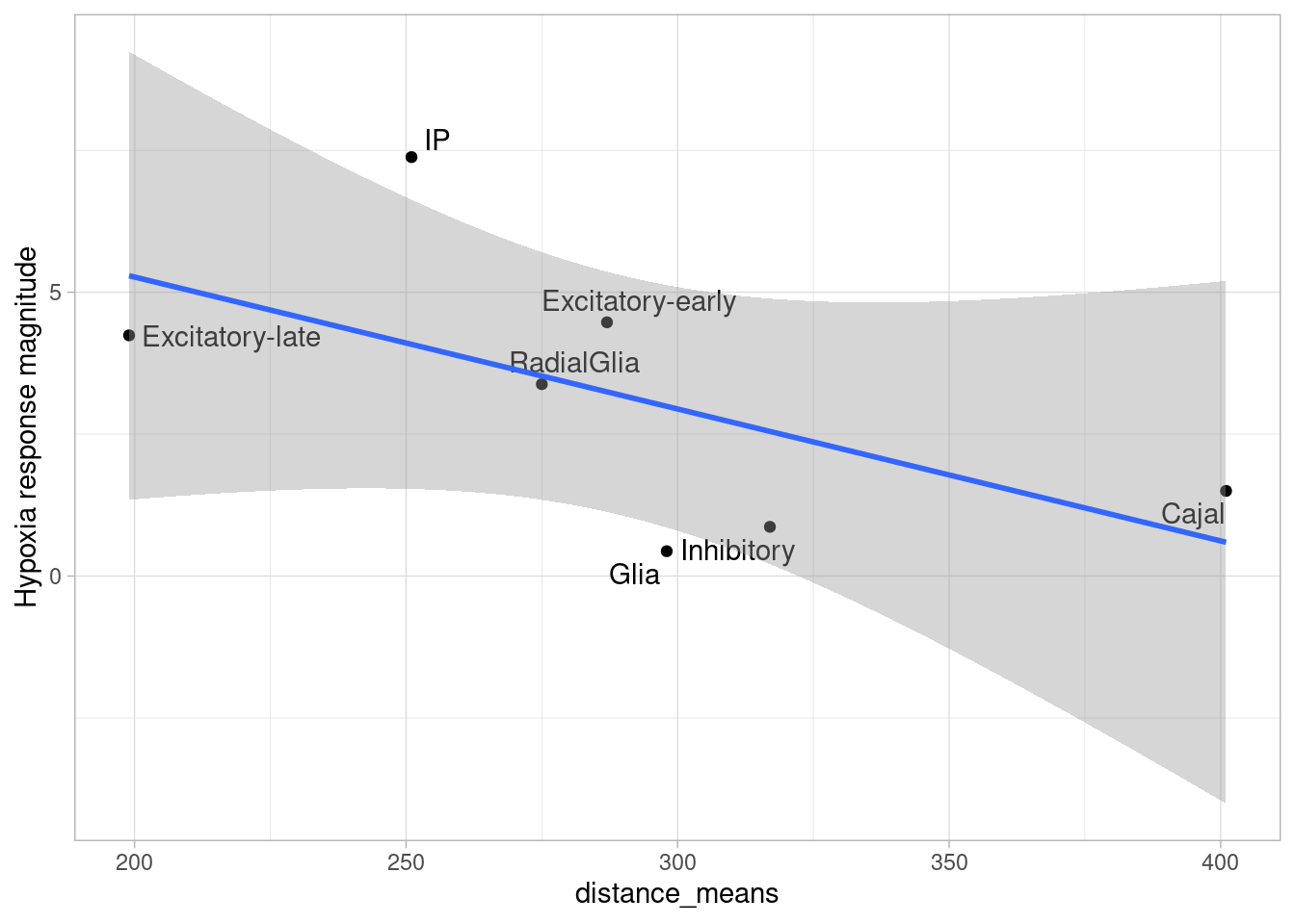

ggplot(temp, aes(x=distance_medians, y=order, label=celltype)) + geom_point() + geom_text_repel() + geom_smooth(method="lm") + theme_light() + ylab("Hypoxia response magnitude")

`geom_smooth()` using formula = 'y ~ x'

Warning: The following aesthetics were dropped during statistical transformation: label
ℹ This can happen when ggplot fails to infer the correct grouping structure in
  the data.
ℹ Did you forget to specify a `group` aesthetic or to convert a numerical
  variable into a factor?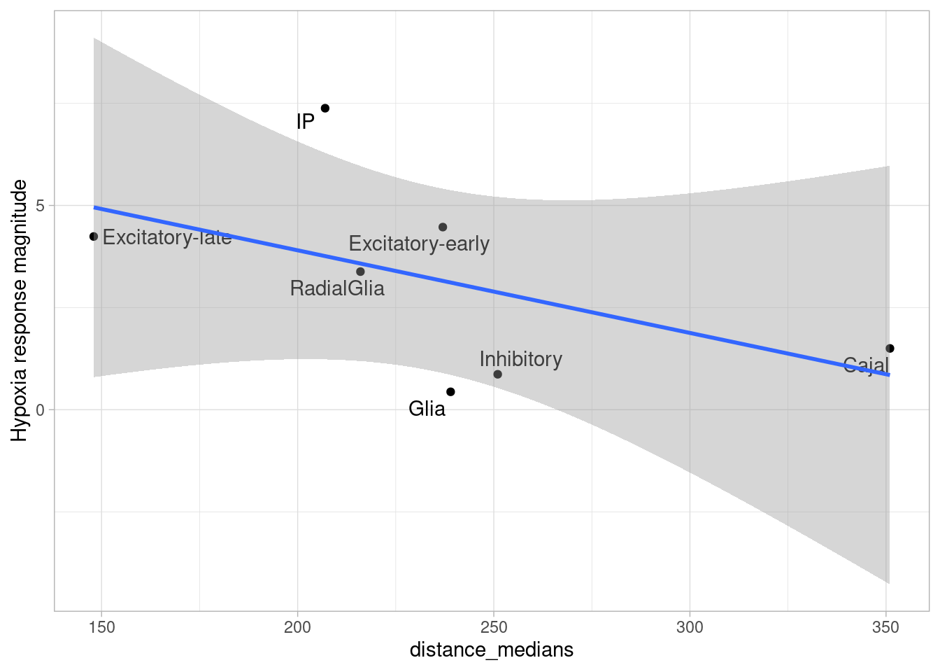

summary(lm(order ~ distance_means, data = temp))

Call:
lm(formula = order ~ distance_means, data = temp)

Residuals:
      1       2       3       4       5       6       7 
 0.9041 -2.5516 -1.0503  3.2981  1.2248 -1.6810 -0.1441 

Coefficients:
               Estimate Std. Error t value Pr(>|t|)  
(Intercept)     9.91510    4.22254   2.348   0.0657 .
distance_means -0.02324    0.01430  -1.626   0.1650  
---
Signif. codes:  0 '***' 0.001 '**' 0.01 '*' 0.05 '.' 0.1 ' ' 1

Residual standard error: 2.175 on 5 degrees of freedom
Multiple R-squared:  0.3458,    Adjusted R-squared:  0.2149 
F-statistic: 2.643 on 1 and 5 DF,  p-value: 0.165

summary(lm(order ~ distance_medians, data = temp))

Call:
lm(formula = order ~ distance_medians, data = temp)

Residuals:
      1       2       3       4       5       6       7 
 0.6523 -2.6748 -0.7132  3.6200  1.3167 -2.0031 -0.1980 

Coefficients:
                 Estimate Std. Error t value Pr(>|t|)  
(Intercept)       7.94637    3.75663   2.115    0.088 .
distance_medians -0.02022    0.01551  -1.304    0.249  
---
Signif. codes:  0 '***' 0.001 '**' 0.01 '*' 0.05 '.' 0.1 ' ' 1

Residual standard error: 2.323 on 5 degrees of freedom
Multiple R-squared:  0.2539,    Adjusted R-squared:  0.1047 
F-statistic: 1.701 on 1 and 5 DF,  p-value: 0.2489

This relationship also holds at the individual level, where distance and response magnitude do not consistently correlate across individuals for a given cell type.

Session information

sessionInfo()

R version 4.2.0 (2022-04-22)
Platform: x86_64-pc-linux-gnu (64-bit)
Running under: CentOS Linux 7 (Core)

Matrix products: default
BLAS/LAPACK: /software/openblas-0.3.13-el7-x86_64/lib/libopenblas_haswellp-r0.3.13.so

locale:
 [1] LC_CTYPE=en_US.UTF-8 LC_NUMERIC=C         LC_TIME=C           
 [4] LC_COLLATE=C         LC_MONETARY=C        LC_MESSAGES=C       
 [7] LC_PAPER=C           LC_NAME=C            LC_ADDRESS=C        
[10] LC_TELEPHONE=C       LC_MEASUREMENT=C     LC_IDENTIFICATION=C 

attached base packages:
[1] stats     graphics  grDevices utils     datasets  methods   base     

other attached packages:
 [1] emmeans_1.7.3            afex_1.3-1               lme4_1.1-35.1           
 [4] Matrix_1.6-3             fgsea_1.22.0             flashier_1.0.7          
 [7] magrittr_2.0.3           ebnm_1.1-2               mixsqp_0.3-48           
[10] flashr_0.6-8             knitr_1.45               ggrepel_0.9.4           
[13] pheatmap_1.0.12          udr_0.3-153              mashr_0.2.79            
[16] ashr_2.2-63              ggbreak_0.1.2            RColorBrewer_1.1-3      
[19] pals_1.8                 lubridate_1.9.3          forcats_1.0.0           
[22] stringr_1.5.0            dplyr_1.1.4              purrr_1.0.2             
[25] readr_2.1.4              tidyr_1.3.0              tibble_3.2.1            
[28] tidyverse_2.0.0          SeuratObject_4.1.4       Seurat_4.4.0            
[31] variancePartition_1.28.9 BiocParallel_1.32.6      ggplot2_3.4.4           
[34] edgeR_3.40.2             limma_3.54.2             workflowr_1.7.0         

loaded via a namespace (and not attached):
  [1] estimability_1.3       scattermore_1.2        coda_0.19-4           
  [4] bit64_4.0.5            multcomp_1.4-19        irlba_2.3.5.1         
  [7] data.table_1.14.8      doParallel_1.0.17      generics_0.1.3        
 [10] BiocGenerics_0.44.0    TH.data_1.1-1          callr_3.7.3           
 [13] RhpcBLASctl_0.23-42    cowplot_1.1.1          RANN_2.6.1            
 [16] future_1.33.1          bit_4.0.5              tzdb_0.4.0            
 [19] horseshoe_0.2.0        spatstat.data_3.0-3    httpuv_1.6.5          
 [22] assertthat_0.2.1       xfun_0.41              hms_1.1.3             
 [25] jquerylib_0.1.4        evaluate_0.23          promises_1.2.0.1      
 [28] fansi_1.0.5            progress_1.2.2         caTools_1.18.2        
 [31] igraph_1.5.1           htmlwidgets_1.6.2      spatstat.geom_3.2-7   
 [34] deconvolveR_1.2-1      ellipsis_0.3.2         backports_1.4.1       
 [37] aod_1.3.2              deldir_1.0-6           vctrs_0.6.4           
 [40] Biobase_2.58.0         ROCR_1.0-11            abind_1.4-5           
 [43] cachem_1.0.8           withr_2.5.2            progressr_0.14.0      
 [46] vroom_1.6.4            sctransform_0.4.1      prettyunits_1.1.1     
 [49] goftest_1.2-3          softImpute_1.4-1       cluster_2.1.3         
 [52] pacman_0.5.1           lazyeval_0.2.2         crayon_1.5.2          
 [55] spatstat.explore_3.0-6 pkgconfig_2.0.3        labeling_0.4.3        
 [58] nlme_3.1-157           rlang_1.1.3            globals_0.16.2        
 [61] lifecycle_1.0.4        miniUI_0.1.1.1         sandwich_3.0-1        
 [64] dichromat_2.0-0.1      invgamma_1.1           rprojroot_2.0.3       
 [67] polyclip_1.10-0        matrixStats_1.1.0      lmtest_0.9-40         
 [70] aplot_0.2.3            carData_3.0-5          boot_1.3-28           
 [73] zoo_1.8-12             whisker_0.4.1          ggridges_0.5.3        
 [76] processx_3.8.2         png_0.1-8              viridisLite_0.4.2     
 [79] bitops_1.0-7           getPass_0.2-2          KernSmooth_2.23-20    
 [82] SQUAREM_2021.1         parallelly_1.37.0      spatstat.random_3.1-3 
 [85] remaCor_0.0.16         gridGraphics_0.5-1     rmeta_3.0             
 [88] scales_1.2.1           memoise_2.0.1          plyr_1.8.9            
 [91] ica_1.0-3              gplots_3.1.3           compiler_4.2.0        
 [94] fitdistrplus_1.1-8     cli_3.6.1              lmerTest_3.1-3        
 [97] listenv_0.9.1          patchwork_1.1.3        pbapply_1.5-0         
[100] ps_1.7.5               mgcv_1.8-40            MASS_7.3-56           
[103] tidyselect_1.2.0       stringi_1.8.1          highr_0.9             
[106] yaml_2.3.5             locfit_1.5-9.8         grid_4.2.0            
[109] sass_0.4.7             fastmatch_1.1-3        tools_4.2.0           
[112] timechange_0.2.0       future.apply_1.11.1    parallel_4.2.0        
[115] rstudioapi_0.17.1      foreach_1.5.2          git2r_0.30.1          
[118] gridExtra_2.3          trust_0.1-8            EnvStats_2.8.1        
[121] farver_2.1.1           Rtsne_0.16             digest_0.6.34         
[124] shiny_1.7.5.1          Rcpp_1.0.12            car_3.1-2             
[127] broom_1.0.5            later_1.3.0            RcppAnnoy_0.0.19      
[130] httr_1.4.7             Rdpack_2.6             colorspace_2.1-0      
[133] fs_1.6.3               tensor_1.5             reticulate_1.34.0     
[136] truncnorm_1.0-9        splines_4.2.0          uwot_0.1.16           
[139] yulab.utils_0.1.0      spatstat.utils_3.0-4   sp_2.1-3              
[142] mapproj_1.2.11         ggplotify_0.1.2        plotly_4.10.0         
[145] xtable_1.8-4           jsonlite_1.8.7         nloptr_2.0.3          
[148] ggfun_0.1.5            R6_2.5.1               pillar_1.9.0          
[151] htmltools_0.5.7        mime_0.12              glue_1.6.2            
[154] fastmap_1.1.1          minqa_1.2.6            codetools_0.2-18      
[157] maps_3.4.0             mvtnorm_1.2-3          utf8_1.2.4            
[160] lattice_0.20-45        bslib_0.5.1            spatstat.sparse_3.0-3 
[163] numDeriv_2016.8-1.1    pbkrtest_0.5.2         leiden_0.4.2          
[166] gtools_3.9.4           survival_3.3-1         rmarkdown_2.26        
[169] munsell_0.5.0          iterators_1.0.14       reshape2_1.4.4        
[172] gtable_0.3.4           rbibutils_2.2.16